9 Case study: analyzing usenet text
In our final chapter, we’ll use what we’ve learned in this book to perform a start-to-finish analysis of a set of 20,000 messages sent to 20 Usenet bulletin boards in 1993. The Usenet bulletin boards in this dataset include newsgroups for topics like politics, religion, cars, sports, and cryptography, and offer a rich set of text written by many users. This data set is publicly available at http://qwone.com/~jason/20Newsgroups/ (the 20news-bydate.tar.gz file) and has become popular for exercises in text analysis and machine learning.
9.1 Pre-processing
We’ll start by reading in all the messages from the 20news-bydate folder, which are organized in sub-folders with one file for each message. We can read in files like these with a combination of read_lines(), map() and unnest().
Note that this step may take several minutes to read all the documents.
training_folder <- "data/20news-bydate/20news-bydate-train/"

# Define a function to read all files from a folder into a data frame
read_folder <- function(infolder) {
  tibble(file = dir(infolder, full.names = TRUE)) %>%
    mutate(text = map(file, read_lines)) %>%
    transmute(id = basename(file), text) %>%
    unnest(text)
}

# Use unnest() and map() to apply read_folder to each subfolder
raw_text <- tibble(folder = dir(training_folder, full.names = TRUE)) %>%
  mutate(folder_out = map(folder, read_folder)) %>%
  unnest(cols = c(folder_out)) %>%
  transmute(newsgroup = basename(folder), id, text)
raw_text
#> # A tibble: 511,655 × 3
#>    newsgroup   id    text
#>    <chr>       <chr> <chr>
#>  1 alt.atheism 49960 "From: mathew <mathew@mantis.co.uk>"
#>  2 alt.atheism 49960 "Subject: Alt.Atheism FAQ: Atheist Resources"
#>  3 alt.atheism 49960 "Summary: Books, addresses, music -- anything related to a…
#>  4 alt.atheism 49960 "Keywords: FAQ, atheism, books, music, fiction, addresses,…
#>  5 alt.atheism 49960 "Expires: Thu, 29 Apr 1993 11:57:19 GMT"
#>  6 alt.atheism 49960 "Distribution: world"
#>  7 alt.atheism 49960 "Organization: Mantis Consultants, Cambridge. UK."
#>  8 alt.atheism 49960 "Supersedes: <19930301143317@mantis.co.uk>"
#>  9 alt.atheism 49960 "Lines: 290"
#> 10 alt.atheism 49960 ""
#> # ℹ 511,645 more rows
Notice the newsgroup column, which describes which of the 20 newsgroups each message comes from, and id column, which identifies a unique message within that newsgroup. What newsgroups are included, and how many messages were posted in each (Figure 9.1)?
library(ggplot2)

raw_text %>%
  group_by(newsgroup) %>%
  summarize(messages = n_distinct(id)) %>%
  ggplot(aes(messages, newsgroup)) +
  geom_col() +
  labs(y = NULL)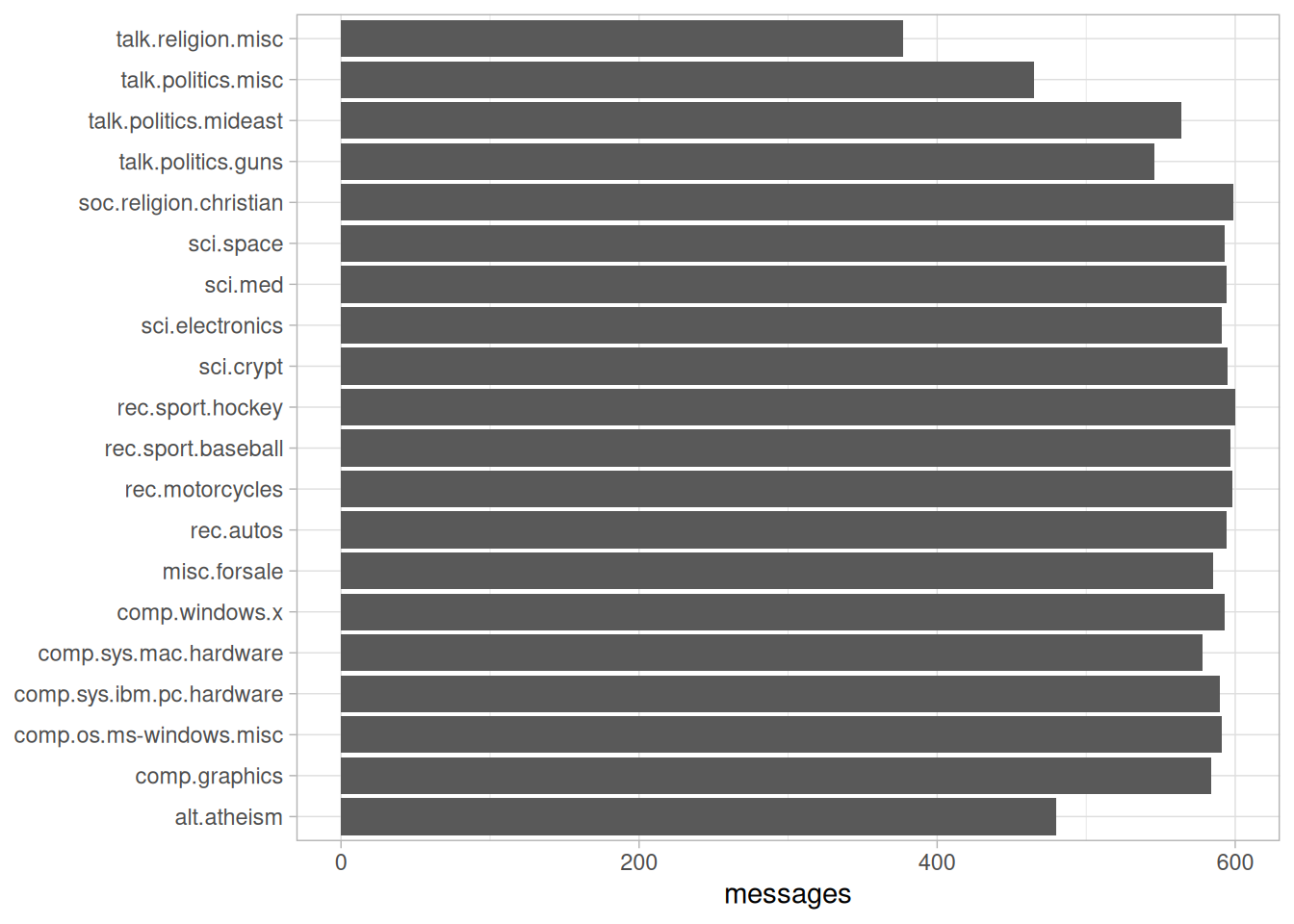
Figure 9.1: Number of messages from each newsgroup
We can see that Usenet newsgroup names are named hierarchically, starting with a main topic such as “talk”, “sci”, or “rec”, followed by further specifications.
9.1.1 Pre-processing text
Most of the datasets we’ve examined in this book were pre-processed, meaning we didn’t have to remove, for example, copyright notices from the Jane Austen novels. Here, however, each message has some structure and extra text that we don’t want to include in our analysis. For example, every message has a header, containing field such as “from:” or “in_reply_to:” that describe the message. Some also have automated email signatures, which occur after a line like --.
This kind of pre-processing can be done within the dplyr package, using a combination of cumsum() (cumulative sum) and str_detect() from stringr.
library(stringr)

# must occur after the first occurrence of an empty line,
# and before the first occurrence of a line starting with --
cleaned_text <- raw_text %>%
  group_by(newsgroup, id) %>%
  filter(cumsum(text == "") > 0,
         cumsum(str_detect(text, "^--")) == 0) %>%
  ungroup()
Many lines also have nested text representing quotes from other users, typically starting with a line like “so-and-so writes…” These can be removed with a few regular expressions.
We also choose to manually remove two messages, 9704 and
9985 that contained a large amount of non-text content.
cleaned_text <- cleaned_text %>%
  filter(str_detect(text, "^[^>]+[A-Za-z\\d]") | text == "",
         !str_detect(text, "writes(:|\\.\\.\\.)$"),
         !str_detect(text, "^In article <"),
         !id %in% c(9704, 9985))
At that point, we’re ready to use unnest_tokens() to split the dataset into tokens, while removing stop-words.
library(tidytext)

usenet_words <- cleaned_text %>%
  unnest_tokens(word, text) %>%
  filter(str_detect(word, "[a-z']$"),
         !word %in% stop_words$word)
Every raw text dataset will require different steps for data cleaning, which will often involve some trial-and-error and exploration of unusual cases in the dataset. It’s important to notice that this cleaning can be achieved using tidy tools such as dplyr and tidyr.
9.2 Words in newsgroups
Now that we’ve removed the headers, signatures, and formatting, we can start exploring common words. For starters, we could find the most common words in the entire dataset, or within particular newsgroups.
usenet_words %>%
  count(word, sort = TRUE)
#> # A tibble: 65,912 × 2
#>    word            n
#>    <chr>       <int>
#>  1 people       3656
#>  2 time         2709
#>  3 god          1627
#>  4 system       1610
#>  5 space        1135
#>  6 windows      1126
#>  7 program      1103
#>  8 bit          1101
#>  9 information  1094
#> 10 government   1084
#> # ℹ 65,902 more rows

words_by_newsgroup <- usenet_words %>%
  count(newsgroup, word, sort = TRUE) %>%
  ungroup()

words_by_newsgroup
#> # A tibble: 173,406 × 3
#>    newsgroup               word          n
#>    <chr>                   <chr>     <int>
#>  1 soc.religion.christian  god         917
#>  2 sci.space               space       902
#>  3 talk.politics.mideast   people      729
#>  4 sci.crypt               key         704
#>  5 comp.os.ms-windows.misc windows     638
#>  6 talk.politics.mideast   armenian    583
#>  7 sci.crypt               db          549
#>  8 talk.politics.mideast   turkish     515
#>  9 rec.autos               car         512
#> 10 talk.politics.mideast   armenians   509
#> # ℹ 173,396 more rows
9.2.1 Finding tf-idf within newsgroups
We’d expect the newsgroups to differ in terms of topic and content, and therefore for the frequency of words to differ between them. Let’s try quantifying this using the tf-idf metric (Chapter 3).
tf_idf <- words_by_newsgroup %>%
  bind_tf_idf(word, newsgroup, n) %>%
  arrange(desc(tf_idf))

tf_idf
#> # A tibble: 173,406 × 6
#>    newsgroup                word               n      tf   idf tf_idf
#>    <chr>                    <chr>          <int>   <dbl> <dbl>  <dbl>
#>  1 comp.sys.ibm.pc.hardware scsi             485 0.0173   1.20 0.0209
#>  2 talk.politics.mideast    armenian         583 0.00805  2.30 0.0185
#>  3 rec.motorcycles          bike             324 0.0137   1.20 0.0165
#>  4 talk.politics.mideast    armenians        509 0.00703  2.30 0.0162
#>  5 sci.crypt                encryption       410 0.00802  1.90 0.0152
#>  6 rec.sport.hockey         hockey           293 0.00815  1.61 0.0131
#>  7 rec.sport.hockey         nhl              157 0.00437  3.00 0.0131
#>  8 talk.politics.misc       stephanopoulos   158 0.00417  3.00 0.0125
#>  9 rec.motorcycles          bikes             97 0.00410  3.00 0.0123
#> 10 comp.windows.x           oname            136 0.00347  3.00 0.0104
#> # ℹ 173,396 more rows
We can examine the top tf-idf for a few selected groups to extract words specific to those topics. For example, we could look at all the sci. boards, visualized in Figure 9.2.
tf_idf %>%
  filter(str_detect(newsgroup, "^sci\\.")) %>%
  group_by(newsgroup) %>%
  slice_max(tf_idf, n = 12) %>%
  ungroup() %>%
  mutate(word = reorder(word, tf_idf)) %>%
  ggplot(aes(tf_idf, word, fill = newsgroup)) +
  geom_col(show.legend = FALSE) +
  facet_wrap(~ newsgroup, scales = "free") +
  labs(x = "tf-idf", y = NULL)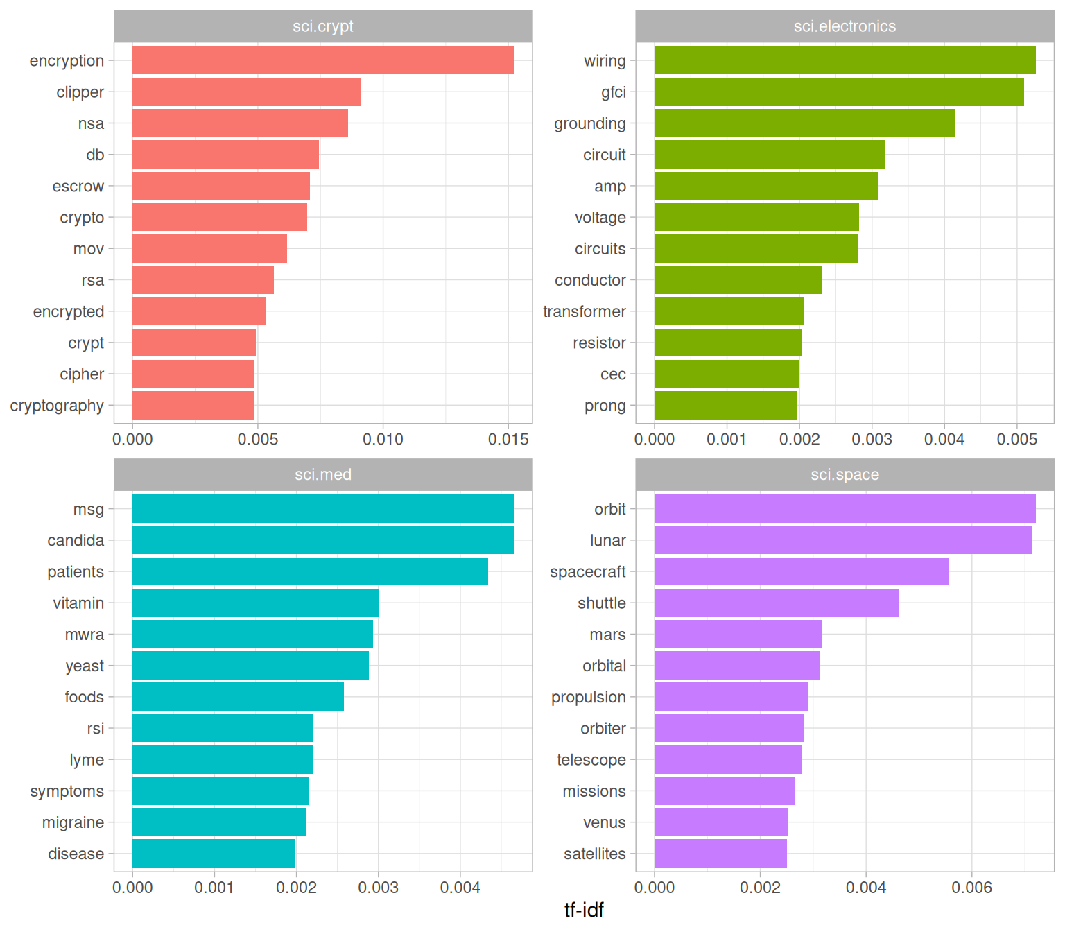
Figure 9.2: Terms with the highest tf-idf within each of the science-related newsgroups
We see lots of characteristic words specific to a particular newsgroup, such as “wiring” and “circuit” on the sci.electronics topic and “orbit” and “lunar” for the space newsgroup. You could use this same code to explore other newsgroups yourself.
What newsgroups tended to be similar to each other in text content? We could discover this by finding the pairwise correlation of word frequencies within each newsgroup, using the pairwise_cor() function from the widyr package (see Chapter 4.2.2).
library(widyr)

newsgroup_cors <- words_by_newsgroup %>%
  pairwise_cor(newsgroup, word, n, sort = TRUE)

newsgroup_cors
#> # A tibble: 380 × 3
#>    item1                    item2                    correlation
#>    <chr>                    <chr>                          <dbl>
#>  1 talk.religion.misc       soc.religion.christian         0.835
#>  2 soc.religion.christian   talk.religion.misc             0.835
#>  3 alt.atheism              talk.religion.misc             0.773
#>  4 talk.religion.misc       alt.atheism                    0.773
#>  5 alt.atheism              soc.religion.christian         0.744
#>  6 soc.religion.christian   alt.atheism                    0.744
#>  7 comp.sys.mac.hardware    comp.sys.ibm.pc.hardware       0.675
#>  8 comp.sys.ibm.pc.hardware comp.sys.mac.hardware          0.675
#>  9 rec.sport.baseball       rec.sport.hockey               0.574
#> 10 rec.sport.hockey         rec.sport.baseball             0.574
#> # ℹ 370 more rows
We could then filter for stronger correlations among newsgroups, and visualize them in a network (Figure (fig:newsgroupcorsnetwork).
library(ggraph)
library(igraph)
set.seed(2017)

newsgroup_cors %>%
  filter(correlation > .4) %>%
  graph_from_data_frame() %>%
  ggraph(layout = "fr") +
  geom_edge_link(aes(alpha = correlation, width = correlation)) +
  geom_node_point(size = 6, color = "lightblue") +
  geom_node_text(aes(label = name), repel = TRUE) +
  theme_void()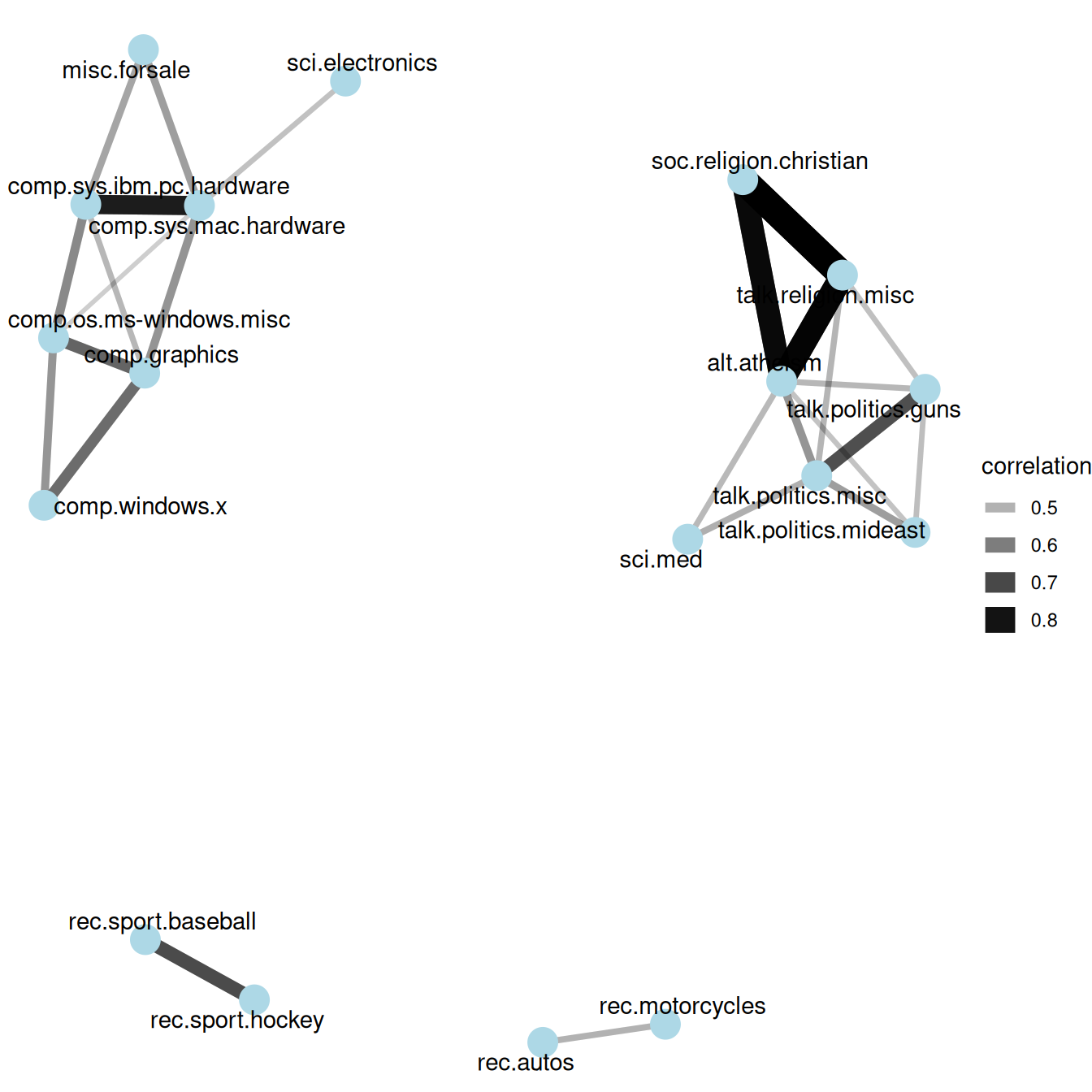
Figure 9.3: A network of Usenet groups based on the correlation of word counts between them, including only connections with a correlation greater than .4
It looks like there were four main clusters of newsgroups: computers/electronics, politics/religion, motor vehicles, and sports. This certainly makes sense in terms of what words and topics we’d expect these newsgroups to have in common.
9.2.2 Topic modeling
In Chapter 6, we used the latent Dirichlet allocation (LDA) algorithm to divide a set of chapters into the books they originally came from. Could LDA do the same to sort out Usenet messages that came from different newsgroups?
Let’s try dividing up messages from the four science-related newsgroups. We first process these into a document-term matrix with cast_dtm() (Chapter 5.2), then fit the model with the LDA() function from the topicmodels package.
# include only words that occur at least 50 times
word_sci_newsgroups <- usenet_words %>%
  filter(str_detect(newsgroup, "^sci")) %>%
  group_by(word) %>%
  mutate(word_total = n()) %>%
  ungroup() %>%
  filter(word_total > 50)

# convert into a document-term matrix
# with document names such as sci.crypt_14147
sci_dtm <- word_sci_newsgroups %>%
  unite(document, newsgroup, id) %>%
  count(document, word) %>%
cast_dtm(document, word, n)What four topics did this model extract, and did they match the four newsgroups? This approach will look familiar from Chapter 6: we visualize each topic based on the most frequent terms within it (Figure 9.4).
sci_lda %>%
  tidy() %>%
  group_by(topic) %>%
  slice_max(beta, n = 8) %>%
  ungroup() %>%
  mutate(term = reorder_within(term, beta, topic)) %>%
  ggplot(aes(beta, term, fill = factor(topic))) +
  geom_col(show.legend = FALSE) +
  facet_wrap(~ topic, scales = "free") +
  scale_y_reordered()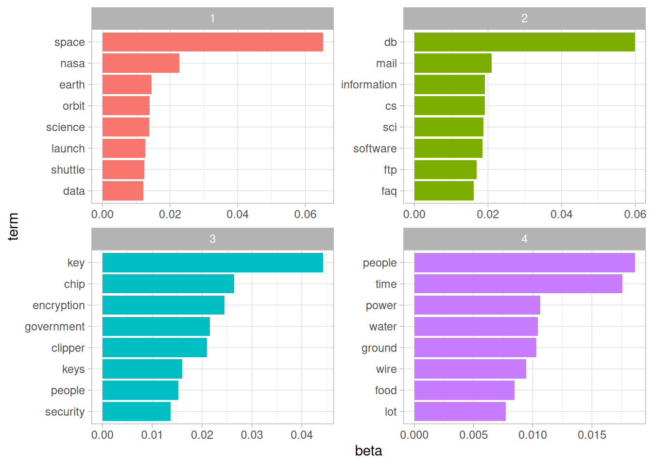
Figure 9.4: Top words from each topic fit by LDA on the science-related newsgroups
From the top words, we can start to suspect which topics may capture which newsgroups. Topic 1 certainly represents the sci.space newsgroup (thus the most common word being “space”), and topic 2 is likely drawn from cryptography, with terms such as “key” and “encryption”. Just as we did in Chapter 6.2.2, we can confirm this by seeing how documents from each newsgroup have higher “gamma” for each topic (Figure 9.5).
sci_lda %>%
  tidy(matrix = "gamma") %>%
  separate(document, c("newsgroup", "id"), sep = "_") %>%
  mutate(newsgroup = reorder(newsgroup, gamma * topic)) %>%
  ggplot(aes(factor(topic), gamma)) +
  geom_boxplot() +
  facet_wrap(~ newsgroup) +
  labs(x = "Topic",
       y = "# of messages where this was the highest % topic")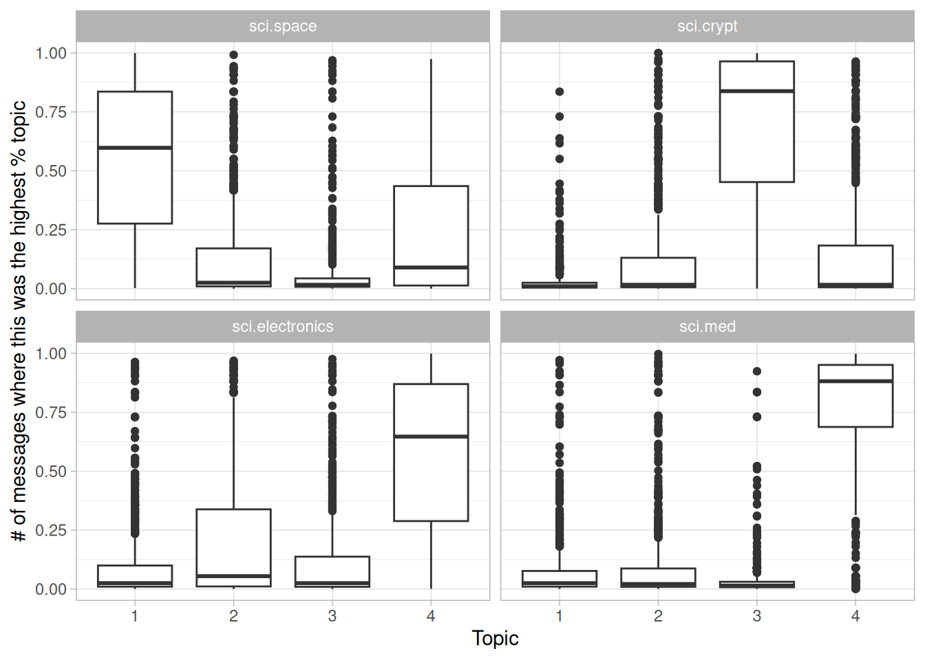
Figure 9.5: Distribution of gamma for each topic within each Usenet newsgroup
Much as we saw in the literature analysis, topic modeling was able to discover the distinct topics present in the text without needing to consult the labels.
Notice that the division of Usenet messages wasn’t as clean as the division of book chapters, with a substantial number of messages from each newsgroup getting high values of “gamma” for other topics. This isn’t surprising since many of the messages are short and could overlap in terms of common words (for example, discussions of space travel could include many of the same words as discussions of electronics). This is a realistic example of how LDA might divide documents into rough topics while still allowing a degree of overlap.
9.3 Sentiment analysis
We can use the sentiment analysis techniques we explored in Chapter 2 to examine how often positive and negative words occurred in these Usenet posts. Which newsgroups were the most positive or negative overall?
In this example we’ll use the AFINN sentiment lexicon, which provides numeric positivity values for each word, and visualize it with a bar plot (Figure 9.6).
newsgroup_sentiments <- words_by_newsgroup %>%
  inner_join(get_sentiments("afinn"), by = "word") %>%
  group_by(newsgroup) %>%
  summarize(value = sum(value * n) / sum(n))

newsgroup_sentiments %>%
  mutate(newsgroup = reorder(newsgroup, value)) %>%
  ggplot(aes(value, newsgroup, fill = value > 0)) +
  geom_col(show.legend = FALSE) +
  labs(x = "Average sentiment value", y = NULL)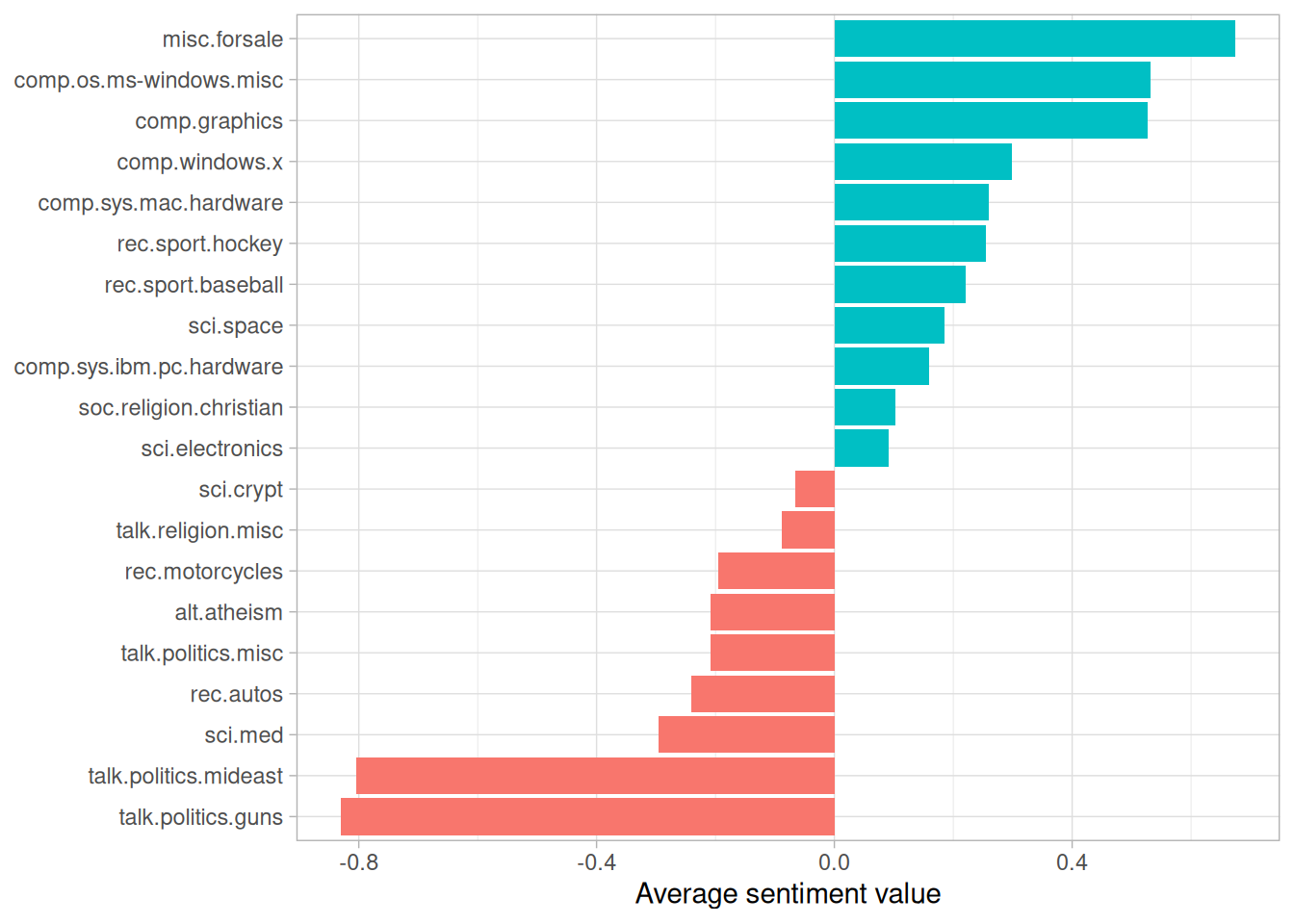
Figure 9.6: Average AFINN value for posts within each newsgroup
According to this analysis, the “misc.forsale” newsgroup was the most positive. This makes sense, since it likely included many positive adjectives about the products that users wanted to sell!
9.3.1 Sentiment analysis by word
It’s worth looking deeper to understand why some newsgroups ended up more positive or negative than others. For that, we can examine the total positive and negative contributions of each word.
contributions <- usenet_words %>%
  inner_join(get_sentiments("afinn"), by = "word") %>%
  group_by(word) %>%
  summarize(occurences = n(),
            contribution = sum(value))
What are these contributions?
contributions
#> # A tibble: 1,909 × 3
#>    word      occurences contribution
#>    <chr>          <int>        <dbl>
#>  1 abandon           13          -26
#>  2 abandoned         19          -38
#>  3 abandons           3           -6
#>  4 abduction          2           -4
#>  5 abhor              4          -12
#>  6 abhorred           1           -3
#>  7 abhorrent          2           -6
#>  8 abilities         16           32
#>  9 ability          177          354
#> 10 aboard             8            8
#> # ℹ 1,899 more rows
Which words had the most effect on sentiment values overall (Figure 9.7)?
contributions %>%
  slice_max(abs(contribution), n = 25) %>%
  mutate(word = reorder(word, contribution)) %>%
  ggplot(aes(contribution, word, fill = contribution > 0)) +
  geom_col(show.legend = FALSE) +
  labs(y = NULL)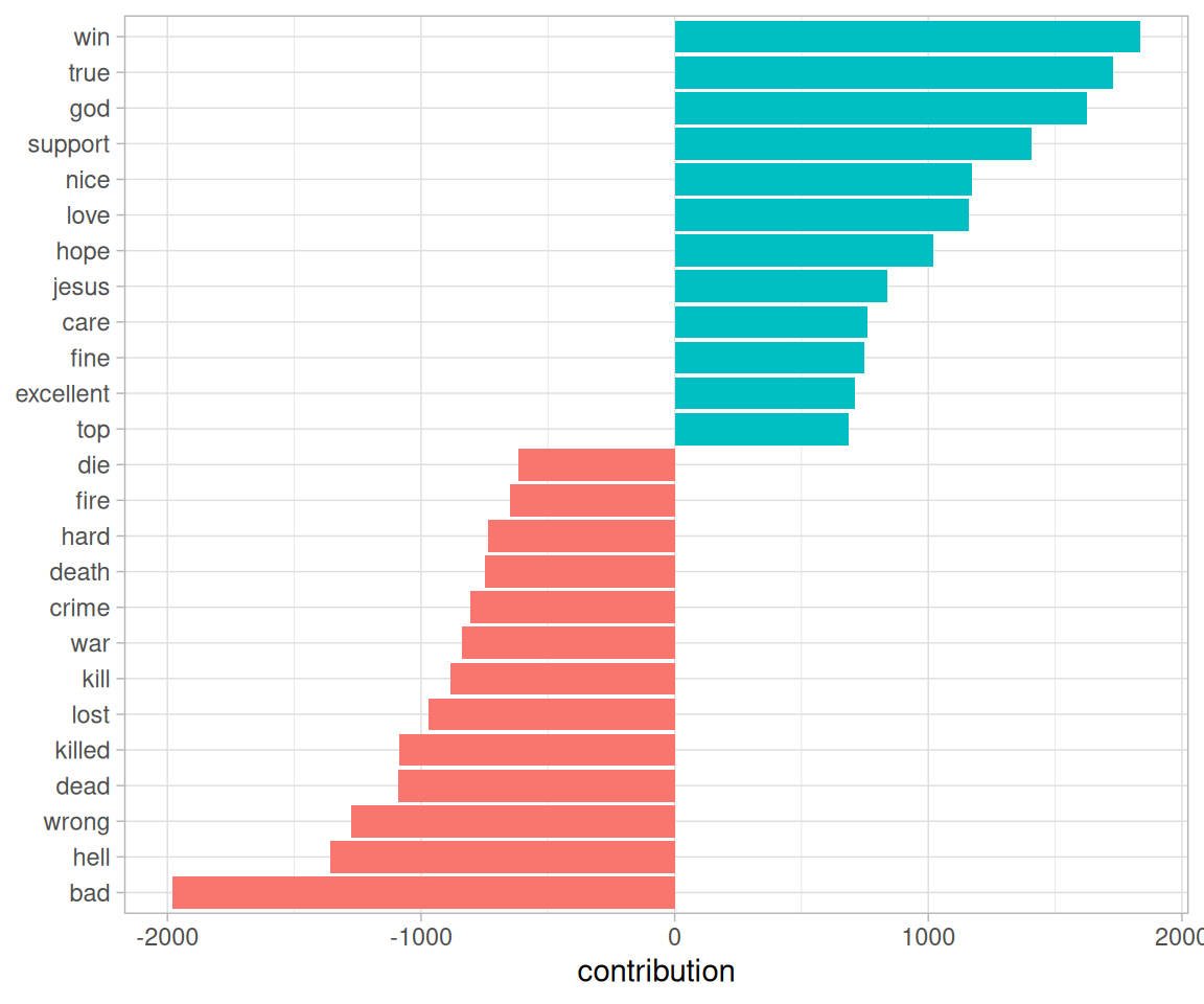
Figure 9.7: Words with the greatest contributions to positive/negative sentiment values in the Usenet text
These words look generally reasonable as indicators of each message’s sentiment, but we can spot possible problems with the approach. “True” could just as easily be a part of “not true” or a similar negative expression, and the words “God” and “Jesus” are apparently very common on Usenet but could easily be used in many contexts, positive or negative.
We may also care about which words contributed the most within each newsgroup, so that we can see which newsgroups might be incorrectly estimated.
top_sentiment_words <- words_by_newsgroup %>%
  inner_join(get_sentiments("afinn"), by = "word") %>%
  mutate(contribution = value * n / sum(n))
We can calculate each word’s contribution to each newsgroup’s sentiment score, and visualize the strongest contributors from a selection of the groups (Figure 9.8).
top_sentiment_words
#> # A tibble: 13,078 × 5
#>    newsgroup              word       n value contribution
#>    <chr>                  <chr>  <int> <dbl>        <dbl>
#>  1 soc.religion.christian god      917     1      0.0144
#>  2 soc.religion.christian jesus    440     1      0.00690
#>  3 talk.politics.guns     gun      425    -1     -0.00667
#>  4 talk.religion.misc     god      296     1      0.00464
#>  5 alt.atheism            god      268     1      0.00421
#>  6 soc.religion.christian faith    257     1      0.00403
#>  7 talk.religion.misc     jesus    256     1      0.00402
#>  8 talk.politics.mideast  killed   202    -3     -0.00951
#>  9 talk.politics.mideast  war      187    -2     -0.00587
#> 10 soc.religion.christian true     179     2      0.00562
#> # ℹ 13,068 more rows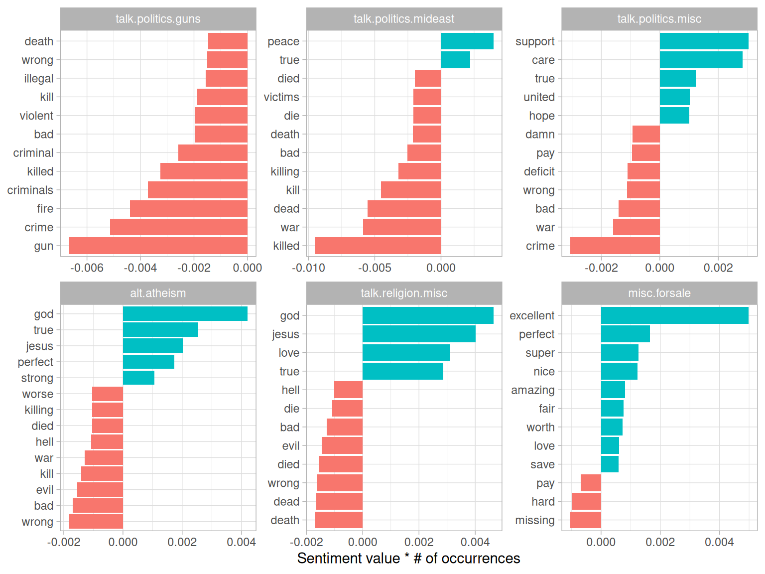
Figure 9.8: Words that contributed the most to sentiment scores within each of six newsgroups
This confirms our hypothesis about the “misc.forsale” newsgroup: most of the sentiment was driven by positive adjectives such as “excellent” and “perfect”. We can also see how much sentiment is confounded with topic. An atheism newsgroup is likely to discuss “god” in detail even in a negative context, and we can see that it makes the newsgroup look more positive. Similarly, the negative contribution of the word “gun” to the “talk.politics.guns” group will occur even when the members are discussing guns positively.
This helps remind us that sentiment analysis can be confounded by topic, and that we should always examine the influential words before interpreting it too deeply.
9.3.2 Sentiment analysis by message
We can also try finding the most positive and negative individual messages, by grouping and summarizing by id rather than newsgroup.
sentiment_messages <- usenet_words %>%
  inner_join(get_sentiments("afinn"), by = "word") %>%
  group_by(newsgroup, id) %>%
  summarize(sentiment = mean(value),
            words = n()) %>%
  ungroup() %>%
  filter(words >= 5)
As a simple measure to reduce the role of randomness, we filtered out messages that had fewer than five words that contributed to sentiment.
What were the most positive messages?
sentiment_messages %>%
  arrange(desc(sentiment))
#> # A tibble: 3,564 × 4
#>    newsgroup               id     sentiment words
#>    <chr>                   <chr>      <dbl> <int>
#>  1 rec.sport.hockey        53560       3.89    18
#>  2 rec.sport.hockey        53602       3.83    30
#>  3 rec.sport.hockey        53822       3.83     6
#>  4 comp.windows.x          66905       3.32    19
#>  5 comp.windows.x          66906       3.32    19
#>  6 comp.os.ms-windows.misc 9904        3.29     7
#>  7 rec.sport.hockey        53645       3.23    13
#>  8 rec.autos               102768      3.2      5
#>  9 misc.forsale            75965       3        5
#> 10 misc.forsale            76037       3        5
#> # ℹ 3,554 more rows
Let’s check this by looking at the most positive message in the whole dataset. To assist in this we could write a short function for printing a specified message.
print_message <- function(group, message_id) {
  result <- cleaned_text %>%
    filter(newsgroup == group, id == message_id, text != "")

  cat(result$text, sep = "\n")
}

print_message("rec.sport.hockey", 53560)
#> Everybody.  Please send me your predictions for the Stanley Cup Playoffs!
#> I want to see who people think will win.!!!!!!!
#> Please Send them in this format, or something comparable:
#> 1. Winner of Buffalo-Boston
#> 2. Winner of Montreal-Quebec
#> 3. Winner of Pittsburgh-New York
#> 4. Winner of New Jersey-Washington
#> 5. Winner of Chicago-(Minnesota/St.Louis)
#> 6. Winner of Toronto-Detroit
#> 7. Winner of Vancouver-Winnipeg
#> 8. Winner of Calgary-Los Angeles
#> 9. Winner of Adams Division (1-2 above)
#> 10. Winner of Patrick Division (3-4 above)
#> 11. Winner of Norris Division (5-6 above)
#> 12. Winner of Smythe Division (7-8 above)
#> 13. Winner of Wales Conference (9-10 above)
#> 14. Winner of Campbell Conference (11-12 above)
#> 15. Winner of Stanley Cup (13-14 above)
#> I will summarize the predictions, and see who is the biggest
#> INTERNET GURU PREDICTING GUY/GAL.
#> Send entries to Richard Madison
#> rrmadiso@napier.uwaterloo.ca
#> PS:  I will send my entries to one of you folks so you know when I say
#> I won, that I won!!!!!
It looks like this message was chosen because it uses the word “winner” many times. How about the most negative message? Turns out it’s also from the hockey site, but has a very different attitude.
sentiment_messages %>%
  arrange(sentiment)
#> # A tibble: 3,564 × 4
#>    newsgroup             id     sentiment words
#>    <chr>                 <chr>      <dbl> <int>
#>  1 rec.sport.hockey      53907      -3        6
#>  2 sci.electronics       53899      -3        5
#>  3 talk.politics.mideast 75918      -3        7
#>  4 rec.autos             101627     -2.83     6
#>  5 comp.graphics         37948      -2.8      5
#>  6 comp.windows.x        67204      -2.7     10
#>  7 talk.politics.guns    53362      -2.67     6
#>  8 alt.atheism           51309      -2.6      5
#>  9 comp.sys.mac.hardware 51513      -2.6      5
#> 10 rec.autos             102883     -2.6      5
#> # ℹ 3,554 more rows

print_message("rec.sport.hockey", 53907)
#> Losers like us? You are the fucking moron who has never heard of the Western
#> Business School, or the University of Western Ontario for that matter. Why
#> don't you pull your head out of your asshole and smell something other than
#> shit for once so you can look on a map to see where UWO is! Back to hockey,
#> the North Stars should be moved because for the past few years they have
#> just been SHIT. A real team like Toronto would never be moved!!!
#> Andrew--
Well, we can confidently say that the sentiment analysis worked!
9.3.3 N-gram analysis
In Chapter 4, we considered the effect of words such as “not” and “no” on sentiment analysis of Jane Austen novels, such as considering whether a phrase like “don’t like” led to passages incorrectly being labeled as positive. The Usenet dataset is a much larger corpus of more modern text, so we may be interested in how sentiment analysis may be reversed in this text.
We’d start by finding and counting all the bigrams in the Usenet posts.
usenet_bigrams <- cleaned_text %>%
  unnest_tokens(bigram, text, token = "ngrams", n = 2)
usenet_bigram_counts <- usenet_bigrams %>%
  count(newsgroup, bigram, sort = TRUE) %>%
  separate(bigram, c("word1", "word2"), sep = " ")
We could then define a list of six words that we suspect are used in negation, such as “no”, “not”, and “without”, and visualize the sentiment-associated words that most often followed them (Figure 9.9). This shows the words that most often contributed in the “wrong” direction.
negate_words <- c("not", "without", "no", "can't", "don't", "won't")

usenet_bigram_counts %>%
  filter(word1 %in% negate_words) %>%
  count(word1, word2, wt = n, sort = TRUE) %>%
  inner_join(get_sentiments("afinn"), by = c(word2 = "word")) %>%
  mutate(contribution = value * n) %>%
  group_by(word1) %>%
  slice_max(abs(contribution), n = 10) %>%
  ungroup() %>%
  mutate(word2 = reorder_within(word2, contribution, word1)) %>%
  ggplot(aes(contribution, word2, fill = contribution > 0)) +
  geom_col(show.legend = FALSE) +
  facet_wrap(~ word1, scales = "free", nrow = 3) +
  scale_y_reordered() +
  labs(x = "Sentiment value * # of occurrences",
       y = "Words preceded by a negation")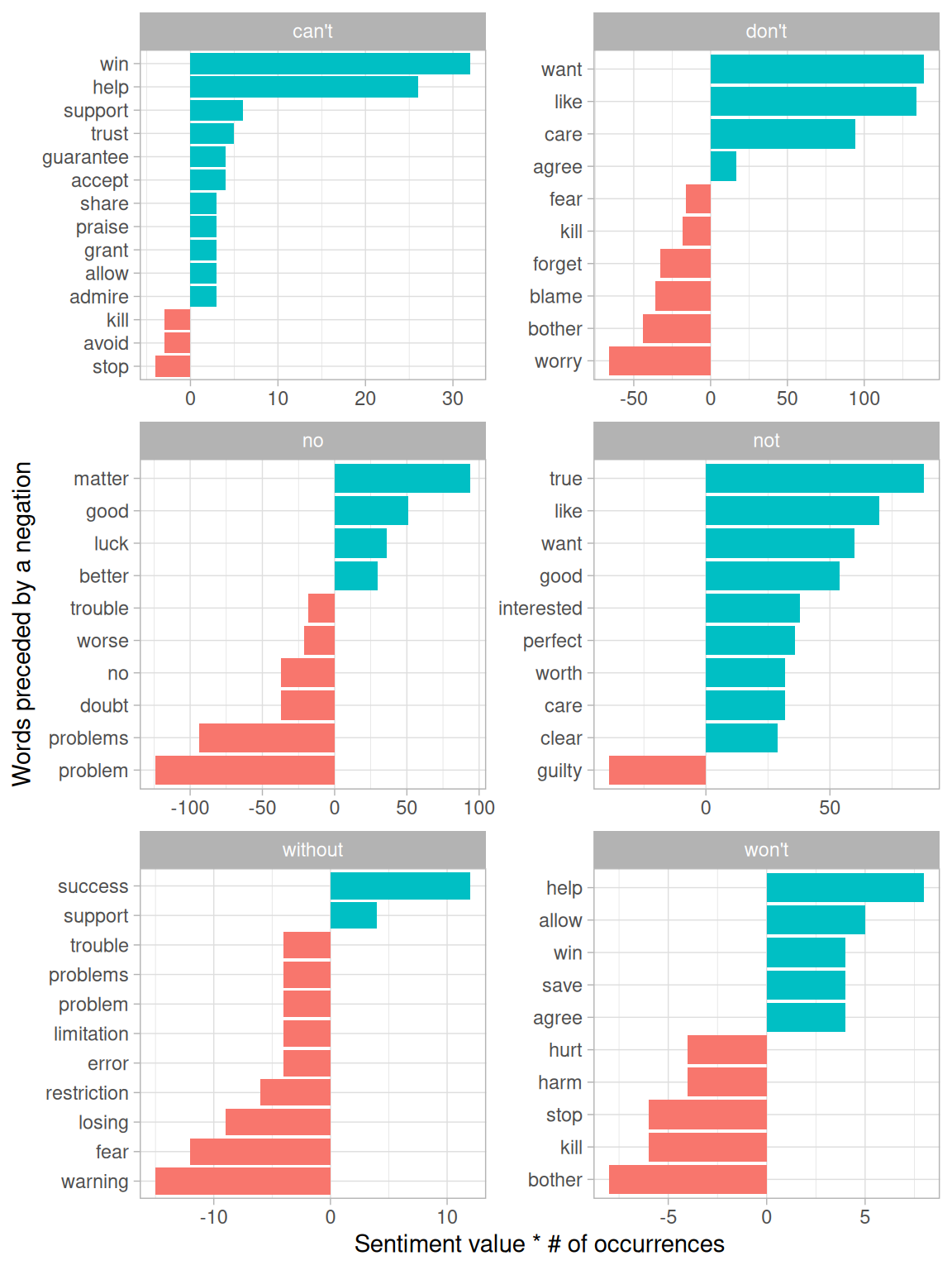
Figure 9.9: Words that contributed the most to sentiment when they followed a ‘negating’ word
It looks like the largest sources of misidentifying a word as positive come from “don’t want/like/care”, and the largest source of incorrectly classified negative sentiment is “no problem”.
9.4 Summary
In this analysis of Usenet messages, we’ve incorporated almost every method for tidy text mining described in this book, ranging from tf-idf to topic modeling and from sentiment analysis to n-gram tokenization. Throughout the chapter, and indeed through all of our case studies, we’ve been able to rely on a small list of common tools for exploration and visualization. We hope that these examples show how much all tidy text analyses have in common with each other, and indeed with all tidy data analyses.