6 Topic modeling
In text mining, we often have collections of documents, such as blog posts or news articles, that we’d like to divide into natural groups so that we can understand them separately. Topic modeling is a method for unsupervised classification of such documents, similar to clustering on numeric data, which finds natural groups of items even when we’re not sure what we’re looking for.
Latent Dirichlet allocation (LDA) is a particularly popular method for fitting a topic model. It treats each document as a mixture of topics, and each topic as a mixture of words. This allows documents to “overlap” each other in terms of content, rather than being separated into discrete groups, in a way that mirrors typical use of natural language.
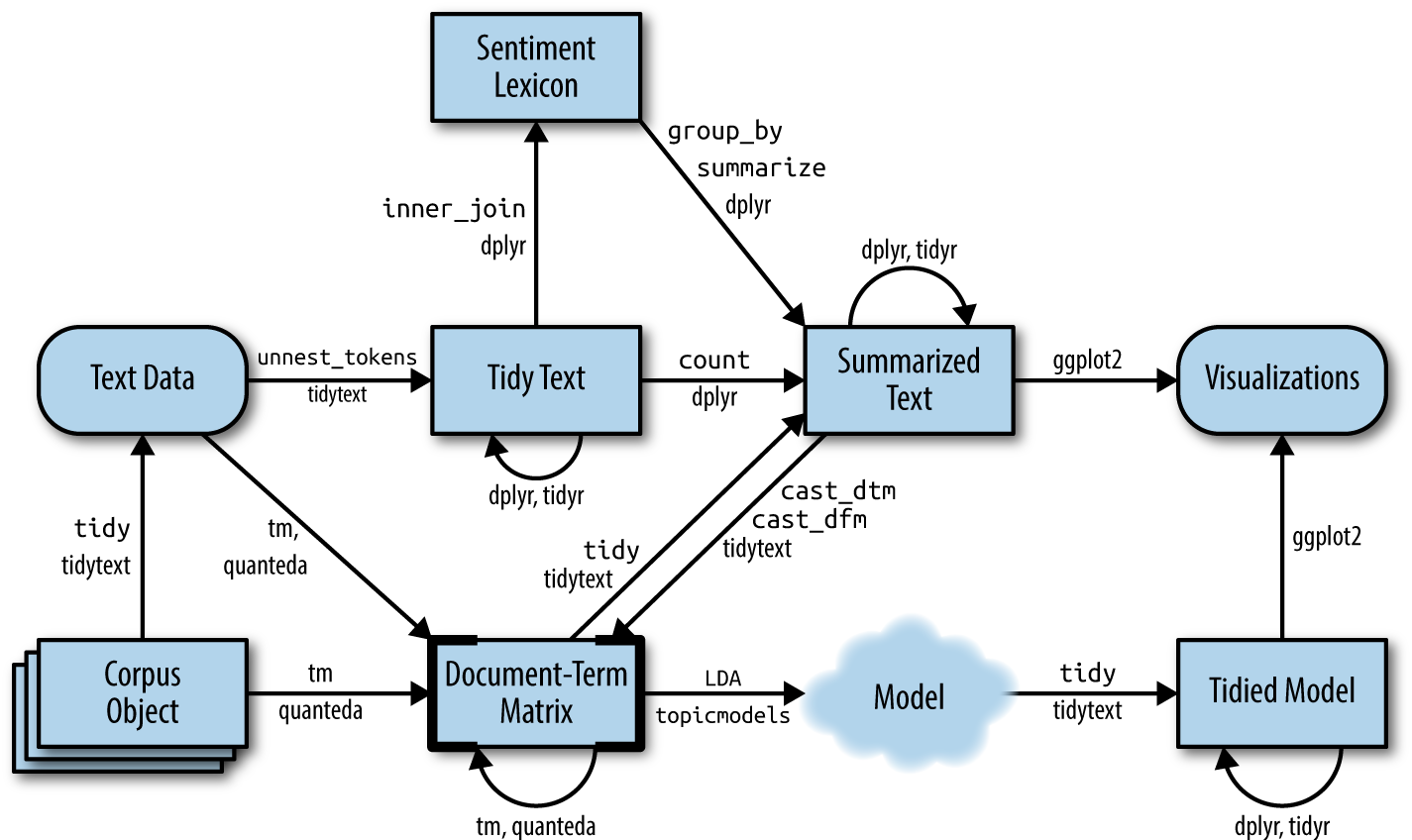
Figure 6.1: A flowchart of a text analysis that incorporates topic modeling. The topicmodels package takes a Document-Term Matrix as input and produces a model that can be tided by tidytext, such that it can be manipulated and visualized with dplyr and ggplot2.
As Figure 6.1 shows, we can use tidy text principles to approach topic modeling with the same set of tidy tools we’ve used throughout this book. In this chapter, we’ll learn to work with LDA objects from the topicmodels package, particularly tidying such models so that they can be manipulated with ggplot2 and dplyr. We’ll also explore an example of clustering chapters from several books, where we can see that a topic model “learns” to tell the difference between the four books based on the text content.
6.1 Latent Dirichlet allocation
Latent Dirichlet allocation is one of the most common algorithms for topic modeling. Without diving into the math behind the model, we can understand it as being guided by two principles.
- Every document is a mixture of topics. We imagine that each document may contain words from several topics in particular proportions. For example, in a two-topic model we could say “Document 1 is 90% topic A and 10% topic B, while Document 2 is 30% topic A and 70% topic B.”
- Every topic is a mixture of words. For example, we could imagine a two-topic model of American news, with one topic for “politics” and one for “entertainment.” The most common words in the politics topic might be “President”, “Congress”, and “government”, while the entertainment topic may be made up of words such as “movies”, “television”, and “actor”. Importantly, words can be shared between topics; a word like “budget” might appear in both equally.
LDA is a mathematical method for estimating both of these at the same time: finding the mixture of words that is associated with each topic, while also determining the mixture of topics that describes each document. There are a number of existing implementations of this algorithm, and we’ll explore one of them in depth.
In Chapter 5 we briefly introduced the AssociatedPress dataset provided by the topicmodels package, as an example of a DocumentTermMatrix. This is a collection of 2246 news articles from an American news agency, mostly published around 1988.
library(topicmodels)

data("AssociatedPress")
AssociatedPress
#> <<DocumentTermMatrix (documents: 2246, terms: 10473)>>
#> Non-/sparse entries: 302031/23220327
#> Sparsity           : 99%
#> Maximal term length: 18
#> Weighting          : term frequency (tf)
We can use the LDA() function from the topicmodels package, setting k = 2, to create a two-topic LDA model.
Almost any topic model in practice will use a larger k,
but we will soon see that this analysis approach extends to a larger
number of topics.
This function returns an object containing the full details of the model fit, such as how words are associated with topics and how topics are associated with documents.
# set a seed so that the output of the model is predictable
ap_lda <- LDA(AssociatedPress, k = 2, control = list(seed = 1234))
ap_lda
#> A LDA_VEM topic model with 2 topics.
Fitting the model was the “easy part”: the rest of the analysis will involve exploring and interpreting the model using tidying functions from the tidytext package.
6.1.1 Word-topic probabilities
In Chapter 5 we introduced the tidy() method, originally from the broom package (Robinson 2017), for tidying model objects. The tidytext package provides this method for extracting the per-topic-per-word probabilities, called \(\beta\) (“beta”), from the model.
library(tidytext)

ap_topics <- tidy(ap_lda, matrix = "beta")
ap_topics
#> # A tibble: 20,946 × 3
#>    topic term           beta
#>    <int> <chr>         <dbl>
#>  1     1 aaron      1.69e-12
#>  2     2 aaron      3.90e- 5
#>  3     1 abandon    2.65e- 5
#>  4     2 abandon    3.99e- 5
#>  5     1 abandoned  1.39e- 4
#>  6     2 abandoned  5.88e- 5
#>  7     1 abandoning 2.45e-33
#>  8     2 abandoning 2.34e- 5
#>  9     1 abbott     2.13e- 6
#> 10     2 abbott     2.97e- 5
#> # ℹ 20,936 more rows
Notice that this has turned the model into a one-topic-per-term-per-row format. For each combination, the model computes the probability of that term being generated from that topic. For example, the term “aaron” has a \(1.686917\times 10^{-12}\) probability of being generated from topic 1, but a \(3.8959408\times 10^{-5}\) probability of being generated from topic 2.
We could use dplyr’s slice_max() to find the 10 terms that are most common within each topic. As a tidy data frame, this lends itself well to a ggplot2 visualization (Figure 6.2).
library(ggplot2)
library(dplyr)

ap_top_terms <- ap_topics %>%
  group_by(topic) %>%
  slice_max(beta, n = 10) %>%
  ungroup() %>%
  arrange(topic, -beta)

ap_top_terms %>%
  mutate(term = reorder_within(term, beta, topic)) %>%
  ggplot(aes(beta, term, fill = factor(topic))) +
  geom_col(show.legend = FALSE) +
  facet_wrap(~ topic, scales = "free") +
  scale_y_reordered()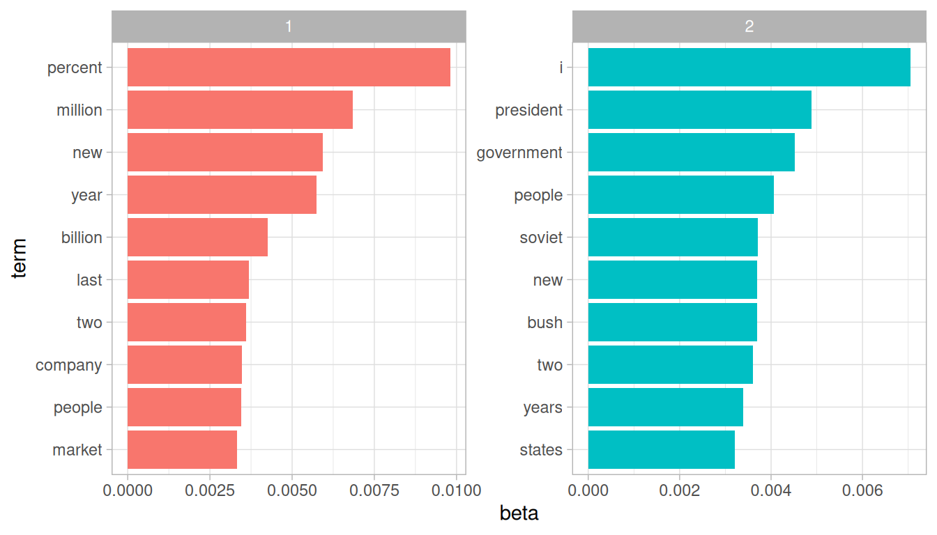
Figure 6.2: The terms that are most common within each topic
This visualization lets us understand the two topics that were extracted from the articles. The most common words in topic 1 include “percent”, “million”, “billion”, and “company”, which suggests it may represent business or financial news. Those most common in topic 2 include “president”, “government”, and “soviet”, suggesting that this topic represents political news. One important observation about the words in each topic is that some words, such as “new” and “people”, are common within both topics. This is an advantage of topic modeling as opposed to “hard clustering” methods: topics used in natural language could have some overlap in terms of words.
As an alternative, we could consider the terms that had the greatest difference in \(\beta\) between topic 1 and topic 2. This can be estimated based on the log ratio of the two: \(\log_2(\frac{\beta_2}{\beta_1})\) (a log ratio is useful because it makes the difference symmetrical: \(\beta_2\) being twice as large leads to a log ratio of 1, while \(\beta_1\) being twice as large results in -1). To constrain it to a set of especially relevant words, we can filter for relatively common words, such as those that have a \(\beta\) greater than 1/1000 in at least one topic.
library(tidyr)

beta_wide <- ap_topics %>%
  mutate(topic = paste0("topic", topic)) %>%
  pivot_wider(names_from = topic, values_from = beta) %>%
  filter(topic1 > .001 | topic2 > .001) %>%
  mutate(log_ratio = log2(topic2 / topic1))

beta_wide
#> # A tibble: 198 × 4
#>    term              topic1      topic2 log_ratio
#>    <chr>              <dbl>       <dbl>     <dbl>
#>  1 administration 0.000431  0.00138         1.68
#>  2 ago            0.00107   0.000842       -0.339
#>  3 agreement      0.000671  0.00104         0.630
#>  4 aid            0.0000476 0.00105         4.46
#>  5 air            0.00214   0.000297       -2.85
#>  6 american       0.00203   0.00168        -0.270
#>  7 analysts       0.00109   0.000000578   -10.9
#>  8 area           0.00137   0.000231       -2.57
#>  9 army           0.000262  0.00105         2.00
#> 10 asked          0.000189  0.00156         3.05
#> # ℹ 188 more rows
The words with the greatest differences between the two topics are visualized in Figure 6.3.
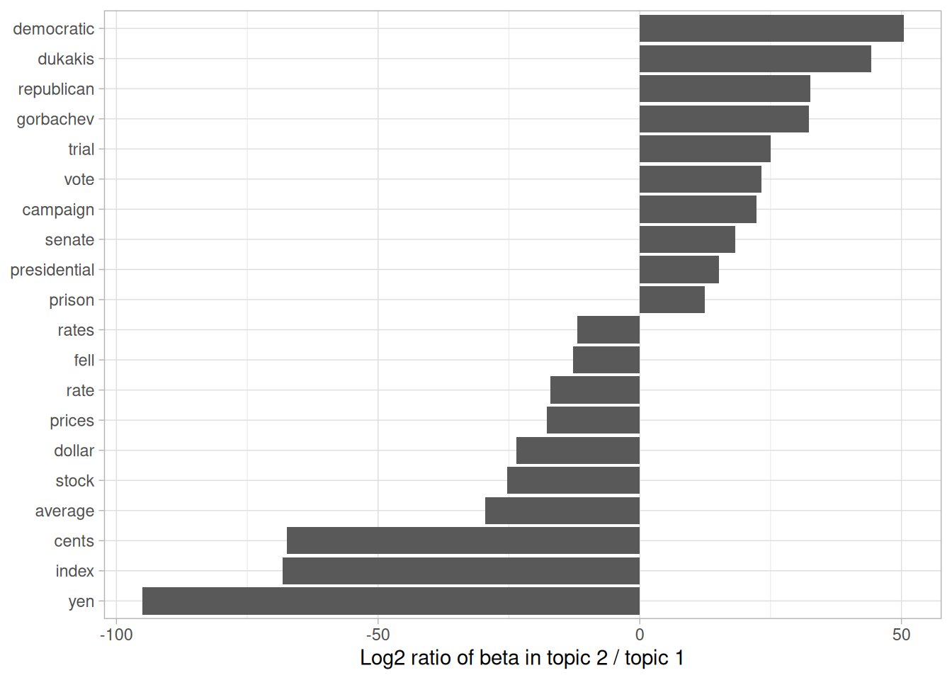
Figure 6.3: Words with the greatest difference in \(\beta\) between topic 2 and topic 1
We can see that the words more common in topic 2 include political parties such as “democratic” and “republican”, as well as politician’s names such as “dukakis” and “gorbachev”. Topic 1 was more characterized by currencies like “yen” and “dollar”, as well as financial terms such as “index”, “prices” and “rates”. This helps confirm that the two topics the algorithm identified were political and financial news.
6.1.2 Document-topic probabilities
Besides estimating each topic as a mixture of words, LDA also models each document as a mixture of topics. We can examine the per-document-per-topic probabilities, called \(\gamma\) (“gamma”), with the matrix = "gamma" argument to tidy().
ap_documents <- tidy(ap_lda, matrix = "gamma")
ap_documents
#> # A tibble: 4,492 × 3
#>    document topic    gamma
#>       <int> <int>    <dbl>
#>  1        1     1 0.248
#>  2        2     1 0.362
#>  3        3     1 0.527
#>  4        4     1 0.357
#>  5        5     1 0.181
#>  6        6     1 0.000588
#>  7        7     1 0.773
#>  8        8     1 0.00445
#>  9        9     1 0.967
#> 10       10     1 0.147
#> # ℹ 4,482 more rows
Each of these values is an estimated proportion of words from that document that are generated from that topic. For example, the model estimates that only about 25% of the words in document 1 were generated from topic 1.
We can see that many of these documents were drawn from a mix of the two topics, but that document 6 was drawn almost entirely from topic 2, having a \(\gamma\) from topic 1 close to zero. To check this answer, we could tidy() the document-term matrix (see Chapter 5.1) and check what the most common words in that document were.
tidy(AssociatedPress) %>%
  filter(document == 6) %>%
  arrange(desc(count))
#> # A tibble: 287 × 3
#>    document term           count
#>       <int> <chr>          <dbl>
#>  1        6 noriega           16
#>  2        6 panama            12
#>  3        6 jackson            6
#>  4        6 powell             6
#>  5        6 administration     5
#>  6        6 economic           5
#>  7        6 general            5
#>  8        6 i                  5
#>  9        6 panamanian         5
#> 10        6 american           4
#> # ℹ 277 more rows
Based on the most common words, this appears to be an article about the relationship between the American government and Panamanian dictator Manuel Noriega, which means the algorithm was right to place it in topic 2 (as political/national news).
6.2 Example: the great library heist
When examining a statistical method, it can be useful to try it on a very simple case where you know the “right answer”. For example, we could collect a set of documents that definitely relate to four separate topics, then perform topic modeling to see whether the algorithm can correctly distinguish the four groups. This lets us double-check that the method is useful, and gain a sense of how and when it can go wrong. We’ll try this with some data from classic literature.
Suppose a vandal has broken into your study and torn apart four of your books:
- Great Expectations by Charles Dickens
- The War of the Worlds by H.G. Wells
- Twenty Thousand Leagues Under the Sea by Jules Verne
- Pride and Prejudice by Jane Austen
This vandal has torn the books into individual chapters, and left them in one large pile. How can we restore these disorganized chapters to their original books? This is a challenging problem since the individual chapters are unlabeled: we don’t know what words might distinguish them into groups. We’ll thus use topic modeling to discover how chapters cluster into distinct topics, each of them (presumably) representing one of the books.
We’ll retrieve the text of these four books using the gutenbergr package introduced in Chapter 3.
titles <- c("Twenty Thousand Leagues under the Sea",
            "The War of the Worlds",
            "Pride and Prejudice",
            "Great Expectations")
library(gutenbergr)

books <- gutenberg_works(title %in% titles) %>%
  gutenberg_download(meta_fields = "title")
As pre-processing, we divide these into chapters, use tidytext’s unnest_tokens() to separate them into words, then remove stop_words. We’re treating every chapter as a separate “document”, each with a name like Great Expectations_1 or Pride and Prejudice_11. (In other applications, each document might be one newspaper article, or one blog post).
library(stringr)

# divide into documents, each representing one chapter
by_chapter <- books %>%
  group_by(title) %>%
  mutate(chapter = cumsum(str_detect(
    text, regex("^chapter ", ignore_case = TRUE)
  ))) %>%
  ungroup() %>%
  filter(chapter > 0) %>%
  unite(document, title, chapter)

# split into words
by_chapter_word <- by_chapter %>%
  unnest_tokens(word, text)

# find document-word counts
word_counts <- by_chapter_word %>%
  anti_join(stop_words) %>%
  count(document, word, sort = TRUE)

word_counts
#> # A tibble: 104,704 × 3
#>    document                 word        n
#>    <chr>                    <chr>   <int>
#>  1 Great Expectations_57    joe        88
#>  2 Great Expectations_7     joe        70
#>  3 Great Expectations_17    biddy      63
#>  4 Great Expectations_27    joe        58
#>  5 Great Expectations_38    estella    58
#>  6 Great Expectations_2     joe        56
#>  7 Great Expectations_23    pocket     53
#>  8 Great Expectations_15    joe        50
#>  9 Great Expectations_18    joe        50
#> 10 The War of the Worlds_16 brother    50
#> # ℹ 104,694 more rows
6.2.1 LDA on chapters
Right now our data frame word_counts is in a tidy form, with one-term-per-document-per-row, but the topicmodels package requires a DocumentTermMatrix. As described in Chapter 5.2, we can cast a one-token-per-row table into a DocumentTermMatrix with tidytext’s cast_dtm().
chapters_dtm <- word_counts %>%
  cast_dtm(document, word, n)

chapters_dtm
#> <<DocumentTermMatrix (documents: 193, terms: 18202)>>
#> Non-/sparse entries: 104704/3408282
#> Sparsity           : 97%
#> Maximal term length: 19
#> Weighting          : term frequency (tf)
We can then use the LDA() function to create a four-topic model. In this case we know we’re looking for four topics because there are four books; in other problems we may need to try a few different values of k.
chapters_lda <- LDA(chapters_dtm, k = 4, control = list(seed = 1234))
chapters_lda
#> A LDA_VEM topic model with 4 topics.
Much as we did on the Associated Press data, we can examine per-topic-per-word probabilities.
chapter_topics <- tidy(chapters_lda, matrix = "beta")
chapter_topics
#> # A tibble: 72,808 × 3
#>    topic term         beta
#>    <int> <chr>       <dbl>
#>  1     1 joe     1.41e- 16
#>  2     2 joe     5.13e- 54
#>  3     3 joe     1.40e-  2
#>  4     4 joe     2.75e- 39
#>  5     1 biddy   3.96e- 22
#>  6     2 biddy   5.72e- 62
#>  7     3 biddy   4.63e-  3
#>  8     4 biddy   3.24e- 47
#>  9     1 estella 4.19e- 18
#> 10     2 estella 2.09e-136
#> # ℹ 72,798 more rows
Notice that this has turned the model into a one-topic-per-term-per-row format. For each combination, the model computes the probability of that term being generated from that topic. For example, the term “joe” has an almost zero probability of being generated from topics 1, 2, or 3, but it makes up 0% of topic 4.
We could use dplyr’s slice_max() to find the top 5 terms within each topic.
top_terms <- chapter_topics %>%
  group_by(topic) %>%
  slice_max(beta, n = 5) %>%
  ungroup() %>%
  arrange(topic, -beta)

top_terms
#> # A tibble: 20 × 3
#>    topic term         beta
#>    <int> <chr>       <dbl>
#>  1     1 people    0.00629
#>  2     1 martians  0.00590
#>  3     1 time      0.00550
#>  4     1 black     0.00501
#>  5     1 night     0.00464
#>  6     2 captain   0.0154
#>  7     2 nautilus  0.0131
#>  8     2 sea       0.00883
#>  9     2 nemo      0.00876
#> 10     2 ned       0.00808
#> 11     3 joe       0.0140
#> 12     3 miss      0.00757
#> 13     3 time      0.00675
#> 14     3 pip       0.00661
#> 15     3 looked    0.00618
#> 16     4 elizabeth 0.0155
#> 17     4 darcy     0.00971
#> 18     4 bennet    0.00765
#> 19     4 miss      0.00764
#> 20     4 jane      0.00714
This tidy output lends itself well to a ggplot2 visualization (Figure 6.4).
library(ggplot2)

top_terms %>%
  mutate(term = reorder_within(term, beta, topic)) %>%
  ggplot(aes(beta, term, fill = factor(topic))) +
  geom_col(show.legend = FALSE) +
  facet_wrap(~ topic, scales = "free") +
  scale_y_reordered()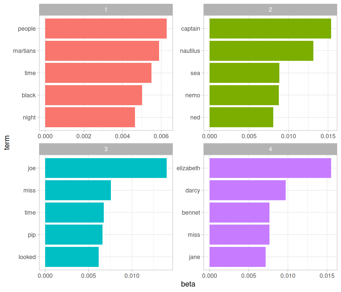
Figure 6.4: The terms that are most common within each topic
These topics are pretty clearly associated with the four books! There’s no question that the topic of “captain”, “nautilus”, “sea”, and “nemo” belongs to Twenty Thousand Leagues Under the Sea, and that “jane”, “darcy”, and “elizabeth” belongs to Pride and Prejudice. We see “pip” and “joe” from Great Expectations and “martians”, “black”, and “night” from The War of the Worlds. We also notice that, in line with LDA being a “fuzzy clustering” method, there can be words in common between multiple topics, such as “miss” in topics 1 and 4, and “time” in topics 3 and 4.
6.2.2 Per-document classification
Each document in this analysis represented a single chapter. Thus, we may want to know which topics are associated with each document. Can we put the chapters back together in the correct books? We can find this by examining the per-document-per-topic probabilities, \(\gamma\) (“gamma”).
chapters_gamma <- tidy(chapters_lda, matrix = "gamma")
chapters_gamma
#> # A tibble: 772 × 3
#>    document                 topic     gamma
#>    <chr>                    <int>     <dbl>
#>  1 Great Expectations_57        1 0.0000134
#>  2 Great Expectations_7         1 0.0000146
#>  3 Great Expectations_17        1 0.0000210
#>  4 Great Expectations_27        1 0.0000190
#>  5 Great Expectations_38        1 0.0000127
#>  6 Great Expectations_2         1 0.0000171
#>  7 Great Expectations_23        1 0.290
#>  8 Great Expectations_15        1 0.0000143
#>  9 Great Expectations_18        1 0.0000126
#> 10 The War of the Worlds_16     1 1.00
#> # ℹ 762 more rows
Each of these values is an estimated proportion of words from that document that are generated from that topic. For example, the model estimates that each word in the Great Expectations_57 document has only a 0% probability of coming from topic 1 (Pride and Prejudice).
Now that we have these topic probabilities, we can see how well our unsupervised learning did at distinguishing the four books. We’d expect that chapters within a book would be found to be mostly (or entirely), generated from the corresponding topic.
First we re-separate the document name into title and chapter, after which we can visualize the per-document-per-topic probability for each (Figure 6.5).
chapters_gamma <- chapters_gamma %>%
  separate(document, c("title", "chapter"), sep = "_", convert = TRUE)

chapters_gamma
#> # A tibble: 772 × 4
#>    title                 chapter topic     gamma
#>    <chr>                   <int> <int>     <dbl>
#>  1 Great Expectations         57     1 0.0000134
#>  2 Great Expectations          7     1 0.0000146
#>  3 Great Expectations         17     1 0.0000210
#>  4 Great Expectations         27     1 0.0000190
#>  5 Great Expectations         38     1 0.0000127
#>  6 Great Expectations          2     1 0.0000171
#>  7 Great Expectations         23     1 0.290
#>  8 Great Expectations         15     1 0.0000143
#>  9 Great Expectations         18     1 0.0000126
#> 10 The War of the Worlds      16     1 1.00
#> # ℹ 762 more rows
# reorder titles in order of topic 1, topic 2, etc before plotting
chapters_gamma %>%
  mutate(title = reorder(title, gamma * topic)) %>%
  ggplot(aes(factor(topic), gamma)) +
  geom_boxplot() +
  facet_wrap(~ title) +
  labs(x = "topic", y = expression(gamma))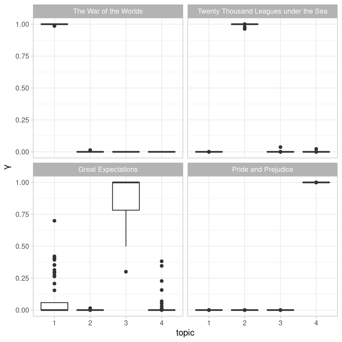
Figure 6.5: The gamma probabilities for each chapter within each book
We notice that almost all of the chapters from Pride and Prejudice, War of the Worlds, and Twenty Thousand Leagues Under the Sea were uniquely identified as a single topic each.
It does look like some chapters from Great Expectations (which should be topic 4) were somewhat associated with other topics. Are there any cases where the topic most associated with a chapter belonged to another book? First we’d find the topic that was most associated with each chapter using slice_max(), which is effectively the “classification” of that chapter.
chapter_classifications <- chapters_gamma %>%
  group_by(title, chapter) %>%
  slice_max(gamma) %>%
  ungroup()

chapter_classifications
#> # A tibble: 193 × 4
#>    title              chapter topic gamma
#>    <chr>                <int> <int> <dbl>
#>  1 Great Expectations       1     3 0.597
#>  2 Great Expectations       2     3 1.00
#>  3 Great Expectations       3     3 0.579
#>  4 Great Expectations       4     3 1.00
#>  5 Great Expectations       5     3 0.647
#>  6 Great Expectations       6     3 1.00
#>  7 Great Expectations       7     3 1.00
#>  8 Great Expectations       8     3 0.994
#>  9 Great Expectations       9     3 1.00
#> 10 Great Expectations      10     3 1.00
#> # ℹ 183 more rows
We can then compare each to the “consensus” topic for each book (the most common topic among its chapters), and see which were most often misidentified.
book_topics <- chapter_classifications %>%
  count(title, topic) %>%
  group_by(title) %>%
  slice_max(n, n = 1) %>%
  ungroup() %>%
  transmute(consensus = title, topic)

chapter_classifications %>%
  inner_join(book_topics, by = "topic") %>%
  filter(title != consensus)
#> # A tibble: 1 × 5
#>   title              chapter topic gamma consensus
#>   <chr>                <int> <int> <dbl> <chr>
#> 1 Great Expectations      54     1 0.700 The War of the Worlds
We see that only two chapters from Great Expectations were misclassified, as LDA described one as coming from the “Pride and Prejudice” topic (topic 1) and one from The War of the Worlds (topic 3). That’s not bad for unsupervised clustering!
6.2.3 By word assignments: augment
One step of the LDA algorithm is assigning each word in each document to a topic. The more words in a document are assigned to that topic, generally, the more weight (gamma) will go on that document-topic classification.
We may want to take the original document-word pairs and find which words in each document were assigned to which topic. This is the job of the augment() function, which also originated in the broom package as a way of tidying model output. While tidy() retrieves the statistical components of the model, augment() uses a model to add information to each observation in the original data.
assignments <- augment(chapters_lda, data = chapters_dtm)
assignments
#> # A tibble: 104,704 × 4
#>    document              term  count .topic
#>    <chr>                 <chr> <dbl>  <dbl>
#>  1 Great Expectations_57 joe      88      3
#>  2 Great Expectations_7  joe      70      3
#>  3 Great Expectations_17 joe       5      3
#>  4 Great Expectations_27 joe      58      3
#>  5 Great Expectations_2  joe      56      3
#>  6 Great Expectations_23 joe       1      3
#>  7 Great Expectations_15 joe      50      3
#>  8 Great Expectations_18 joe      50      3
#>  9 Great Expectations_9  joe      44      3
#> 10 Great Expectations_13 joe      40      3
#> # ℹ 104,694 more rows
This returns a tidy data frame of book-term counts, but adds an extra column: .topic, with the topic each term was assigned to within each document. (Extra columns added by augment always start with ., to prevent overwriting existing columns). We can combine this assignments table with the consensus book titles to find which words were incorrectly classified.
assignments <- assignments %>%
  separate(document, c("title", "chapter"),
           sep = "_", convert = TRUE) %>%
  inner_join(book_topics, by = c(".topic" = "topic"))

assignments
#> # A tibble: 104,704 × 6
#>    title              chapter term  count .topic consensus
#>    <chr>                <int> <chr> <dbl>  <dbl> <chr>
#>  1 Great Expectations      57 joe      88      3 Great Expectations
#>  2 Great Expectations       7 joe      70      3 Great Expectations
#>  3 Great Expectations      17 joe       5      3 Great Expectations
#>  4 Great Expectations      27 joe      58      3 Great Expectations
#>  5 Great Expectations       2 joe      56      3 Great Expectations
#>  6 Great Expectations      23 joe       1      3 Great Expectations
#>  7 Great Expectations      15 joe      50      3 Great Expectations
#>  8 Great Expectations      18 joe      50      3 Great Expectations
#>  9 Great Expectations       9 joe      44      3 Great Expectations
#> 10 Great Expectations      13 joe      40      3 Great Expectations
#> # ℹ 104,694 more rows
This combination of the true book (title) and the book assigned to it (consensus) is useful for further exploration. We can, for example, visualize a confusion matrix, showing how often words from one book were assigned to another, using dplyr’s count() and ggplot2’s geom_tile (Figure 6.6).
library(scales)

assignments %>%
  count(title, consensus, wt = count) %>%
  mutate(across(c(title, consensus), ~str_wrap(., 20))) %>%
  group_by(title) %>%
  mutate(percent = n / sum(n)) %>%
  ggplot(aes(consensus, title, fill = percent)) +
  geom_tile() +
  scale_fill_gradient2(high = "darkred", label = percent_format()) +
  theme_minimal() +
  theme(axis.text.x = element_text(angle = 90, hjust = 1),
        panel.grid = element_blank()) +
  labs(x = "Book words were assigned to",
       y = "Book words came from",
       fill = "% of assignments")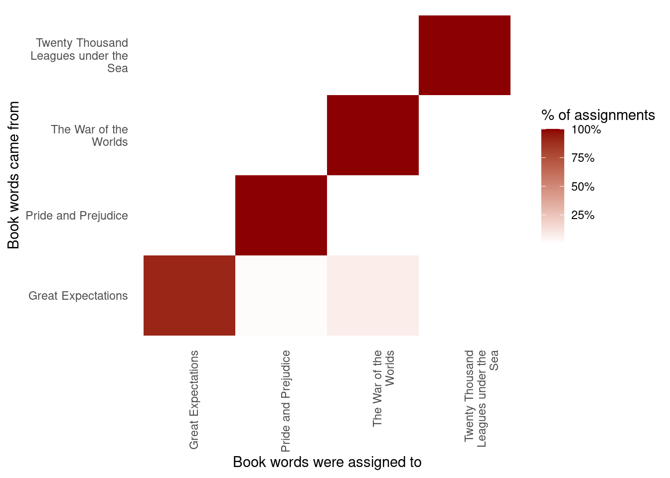
Figure 6.6: Confusion matrix showing where LDA assigned the words from each book. Each row of this table represents the true book each word came from, and each column represents what book it was assigned to.
We notice that almost all the words for Pride and Prejudice, Twenty Thousand Leagues Under the Sea, and War of the Worlds were correctly assigned, while Great Expectations had a fair number of misassigned words (which, as we saw above, led to two chapters getting misclassified).
What were the most commonly mistaken words?
wrong_words <- assignments %>%
  filter(title != consensus)

wrong_words
#> # A tibble: 3,641 × 6
#>    title                                 chapter term     count .topic consensus
#>    <chr>                                   <int> <chr>    <dbl>  <dbl> <chr>
#>  1 Great Expectations                         20 brother      1      1 The War …
#>  2 Great Expectations                         37 brother      2      4 Pride an…
#>  3 Great Expectations                         22 brother      4      4 Pride an…
#>  4 Twenty Thousand Leagues under the Sea       8 miss         1      3 Great Ex…
#>  5 Great Expectations                          5 sergeant    37      1 The War …
#>  6 Great Expectations                         46 captain      1      1 The War …
#>  7 Great Expectations                         32 captain      1      1 The War …
#>  8 The War of the Worlds                      17 captain      5      2 Twenty T…
#>  9 Great Expectations                         54 sea          2      1 The War …
#> 10 Great Expectations                          1 sea          2      1 The War …
#> # ℹ 3,631 more rows

wrong_words %>%
  count(title, consensus, term, wt = count) %>%
  ungroup() %>%
  arrange(desc(n))
#> # A tibble: 2,820 × 4
#>    title              consensus             term         n
#>    <chr>              <chr>                 <chr>    <dbl>
#>  1 Great Expectations The War of the Worlds boat        39
#>  2 Great Expectations The War of the Worlds sergeant    37
#>  3 Great Expectations The War of the Worlds river       34
#>  4 Great Expectations The War of the Worlds jack        28
#>  5 Great Expectations The War of the Worlds tide        28
#>  6 Great Expectations The War of the Worlds water       25
#>  7 Great Expectations The War of the Worlds black       19
#>  8 Great Expectations The War of the Worlds soldiers    19
#>  9 Great Expectations The War of the Worlds london      18
#> 10 Great Expectations The War of the Worlds people      18
#> # ℹ 2,810 more rows
We can see that a number of words were often assigned to the Pride and Prejudice or War of the Worlds cluster even when they appeared in Great Expectations. For some of these words, such as “love” and “lady”, that’s because they’re more common in Pride and Prejudice (we could confirm that by examining the counts).
On the other hand, there are a few wrongly classified words that never appeared in the novel they were misassigned to. For example, we can confirm “flopson” appears only in Great Expectations, even though it’s assigned to the “Pride and Prejudice” cluster.
word_counts %>%
  filter(word == "flopson")
#> # A tibble: 3 × 3
#>   document              word        n
#>   <chr>                 <chr>   <int>
#> 1 Great Expectations_22 flopson    10
#> 2 Great Expectations_23 flopson     7
#> 3 Great Expectations_33 flopson     1
The LDA algorithm is stochastic, and it can accidentally land on a topic that spans multiple books.
6.3 Alternative LDA implementations
The LDA() function in the topicmodels package is only one implementation of the latent Dirichlet allocation algorithm. For example, the mallet package (Mimno 2013) implements a wrapper around the MALLET Java package for text classification tools, and the tidytext package provides tidiers for this model output as well.
The mallet package takes a somewhat different approach to the input format. For instance, it takes non-tokenized documents and performs the tokenization itself, and requires a separate file of stopwords. This means we have to collapse the text into one string for each document before performing LDA.
library(mallet)

# create a vector with one string per chapter
collapsed <- by_chapter_word %>%
  anti_join(stop_words, by = "word") %>%
  mutate(word = str_replace(word, "'", "")) %>%
  group_by(document) %>%
  summarize(text = paste(word, collapse = " "))

# create an empty file of "stopwords"
file.create(empty_file <- tempfile())
docs <- mallet.import(collapsed$document, collapsed$text, empty_file)

mallet_model <- MalletLDA(num.topics = 4)
mallet_model$loadDocuments(docs)
mallet_model$train(100)
Once the model is created, however, we can use the tidy() and augment() functions described in the rest of the chapter in an almost identical way. This includes extracting the probabilities of words within each topic or topics within each document.
# word-topic pairs
tidy(mallet_model)

# document-topic pairs
tidy(mallet_model, matrix = "gamma")

# column needs to be named "term" for "augment"
term_counts <- rename(word_counts, term = word)
augment(mallet_model, term_counts)
We could use ggplot2 to explore and visualize the model in the same way we did the LDA output.
6.4 Summary
This chapter introduces topic modeling for finding clusters of words that characterize a set of documents, and shows how the tidy() verb lets us explore and understand these models using dplyr and ggplot2. This is one of the advantages of the tidy approach to model exploration: the challenges of different output formats are handled by the tidying functions, and we can explore model results using a standard set of tools. In particular, we saw that topic modeling is able to separate and distinguish chapters from four separate books, and explored the limitations of the model by finding words and chapters that it assigned incorrectly.