8 Case study: mining NASA metadata
There are over 32,000 datasets hosted and/or maintained by NASA; these datasets cover topics from Earth science to aerospace engineering to management of NASA itself. We can use the metadata for these datasets to understand the connections between them.
What is metadata? Metadata is a term that refers to data that gives information about other data; in this case, the metadata informs users about what is in these numerous NASA datasets but does not include the content of the datasets themselves.
The metadata includes information like the title of the dataset, a description field, what organization(s) within NASA is responsible for the dataset, keywords for the dataset that have been assigned by a human being, and so forth. NASA places a high priority on making its data open and accessible, even requiring all NASA-funded research to be openly accessible online. The metadata for all its datasets is publicly available online in JSON format.
In this chapter, we will treat the NASA metadata as a text dataset and show how to implement several tidy text approaches with this real-life text. We will use word co-occurrences and correlations, tf-idf, and topic modeling to explore the connections between the datasets. Can we find datasets that are related to each other? Can we find clusters of similar datasets? Since we have several text fields in the NASA metadata, most importantly the title, description, and keyword fields, we can explore the connections between the fields to better understand the complex world of data at NASA. This type of approach can be extended to any domain that deals with text, so let’s take a look at this metadata and get started.
8.1 How data is organized at NASA
First, let’s download the JSON file and take a look at the names of what is stored in the metadata.
#>  [1] "_id"                "@type"              "accessLevel"
#>  [4] "accrualPeriodicity" "bureauCode"         "contactPoint"
#>  [7] "description"        "distribution"       "identifier"
#> [10] "issued"             "keyword"            "landingPage"
#> [13] "language"           "modified"           "programCode"
#> [16] "publisher"          "spatial"            "temporal"
#> [19] "theme"              "title"              "license"
#> [22] "isPartOf"           "references"         "rights"
#> [25] "describedBy"
We see here that we could extract information from who publishes each dataset to what license they are released under.
It seems likely that the title, description, and keywords for each dataset may be most fruitful for drawing connections between datasets. Let’s check them out.
class(metadata$dataset$title)
#> [1] "character"
class(metadata$dataset$description)
#> [1] "character"
class(metadata$dataset$keyword)
#> [1] "list"
The title and description fields are stored as character vectors, but the keywords are stored as a list of character vectors.
8.1.1 Wrangling and tidying the data
Let’s set up separate tidy data frames for title, description, and keyword, keeping the dataset ids for each so that we can connect them later in the analysis if necessary.
library(dplyr)

nasa_title <- tibble(id = metadata$dataset$`_id`$`$oid`,
                     title = metadata$dataset$title)
nasa_title
#> # A tibble: 32,089 × 2
#>    id                       title
#>    <chr>                    <chr>
#>  1 55942a57c63a7fe59b495a77 15 Minute Stream Flow Data: USGS (FIFE)
#>  2 55942a57c63a7fe59b495a78 15 Minute Stream Flow Data: USGS (FIFE)
#>  3 55942a58c63a7fe59b495a79 15 Minute Stream Flow Data: USGS (FIFE)
#>  4 55942a58c63a7fe59b495a7a 2000 Pilot Environmental Sustainability Index (ESI)
#>  5 55942a58c63a7fe59b495a7b 2000 Pilot Environmental Sustainability Index (ESI)
#>  6 55942a58c63a7fe59b495a7c 2000 Pilot Environmental Sustainability Index (ESI)
#>  7 55942a58c63a7fe59b495a7d 2001 Environmental Sustainability Index (ESI)
#>  8 55942a58c63a7fe59b495a7e 2001 Environmental Sustainability Index (ESI)
#>  9 55942a58c63a7fe59b495a7f 2001 Environmental Sustainability Index (ESI)
#> 10 55942a58c63a7fe59b495a80 2001 Environmental Sustainability Index (ESI)
#> # ℹ 32,079 more rows
These are just a few example titles from the datasets we will be exploring. Notice that we have the NASA-assigned ids here, and also that there are duplicate titles on separate datasets.
nasa_desc <- tibble(id = metadata$dataset$`_id`$`$oid`,
                    desc = metadata$dataset$description)

nasa_desc %>%
  select(desc) %>%
  sample_n(5)
#> # A tibble: 5 × 1
#>   desc
#>   <chr>
#> 1 "Preliminary design of aircraft structures is multidisciplinary, involving kn…
#> 2 "Applied Technology Associates (ATA) proposes to develop a new inertial senso…
#> 3 "ML2IWC is the EOS Aura Microwave Limb Sounder (MLS) standard product for clo…
#> 4 "The Cessna Citation II Research aircraft owned and operated by the Universit…
#> 5 "ABSTRACT: Contains in situ diurnal gas exchange and water potential data for…
Here we see the first part of several selected description fields from the metadata.
Now we can build the tidy data frame for the keywords. For this one, we need to use unnest() from tidyr, because they are in a list-column.
library(tidyr)

nasa_keyword <- tibble(id = metadata$dataset$`_id`$`$oid`,
                       keyword = metadata$dataset$keyword) %>%
  unnest(keyword)

nasa_keyword
#> # A tibble: 126,814 × 2
#>    id                       keyword
#>    <chr>                    <chr>
#>  1 55942a57c63a7fe59b495a77 EARTH SCIENCE
#>  2 55942a57c63a7fe59b495a77 HYDROSPHERE
#>  3 55942a57c63a7fe59b495a77 SURFACE WATER
#>  4 55942a57c63a7fe59b495a78 EARTH SCIENCE
#>  5 55942a57c63a7fe59b495a78 HYDROSPHERE
#>  6 55942a57c63a7fe59b495a78 SURFACE WATER
#>  7 55942a58c63a7fe59b495a79 EARTH SCIENCE
#>  8 55942a58c63a7fe59b495a79 HYDROSPHERE
#>  9 55942a58c63a7fe59b495a79 SURFACE WATER
#> 10 55942a58c63a7fe59b495a7a EARTH SCIENCE
#> # ℹ 126,804 more rows
This is a tidy data frame because we have one row for each keyword; this means we will have multiple rows for each dataset because a dataset can have more than one keyword.
Now it is time to use tidytext’s unnest_tokens() for the title and description fields so we can do the text analysis. Let’s also remove stop words from the titles and descriptions. We will not remove stop words from the keywords, because those are short, human-assigned keywords like “RADIATION” or “CLIMATE INDICATORS”.
library(tidytext)

nasa_title <- nasa_title %>%
  unnest_tokens(word, title) %>%
  anti_join(stop_words)

nasa_desc <- nasa_desc %>%
  unnest_tokens(word, desc) %>%
  anti_join(stop_words)
These are now in the tidy text format that we have been working with throughout this book, with one token (word, in this case) per row; let’s take a look before we move on in our analysis.
nasa_title
#> # A tibble: 210,742 × 2
#>    id                       word
#>    <chr>                    <chr>
#>  1 55942a57c63a7fe59b495a77 15
#>  2 55942a57c63a7fe59b495a77 minute
#>  3 55942a57c63a7fe59b495a77 stream
#>  4 55942a57c63a7fe59b495a77 flow
#>  5 55942a57c63a7fe59b495a77 data
#>  6 55942a57c63a7fe59b495a77 usgs
#>  7 55942a57c63a7fe59b495a77 fife
#>  8 55942a57c63a7fe59b495a78 15
#>  9 55942a57c63a7fe59b495a78 minute
#> 10 55942a57c63a7fe59b495a78 stream
#> # ℹ 210,732 more rows
nasa_desc
#> # A tibble: 2,691,556 × 2
#>    id                       word
#>    <chr>                    <chr>
#>  1 55942a57c63a7fe59b495a77 usgs
#>  2 55942a57c63a7fe59b495a77 15
#>  3 55942a57c63a7fe59b495a77 minute
#>  4 55942a57c63a7fe59b495a77 stream
#>  5 55942a57c63a7fe59b495a77 flow
#>  6 55942a57c63a7fe59b495a77 data
#>  7 55942a57c63a7fe59b495a77 kings
#>  8 55942a57c63a7fe59b495a77 creek
#>  9 55942a57c63a7fe59b495a77 konza
#> 10 55942a57c63a7fe59b495a77 prairie
#> # ℹ 2,691,546 more rows
8.1.2 Some initial simple exploration
What are the most common words in the NASA dataset titles? We can use count() from dplyr to check this out.
nasa_title %>%
  count(word, sort = TRUE)
#> # A tibble: 11,607 × 2
#>    word        n
#>    <chr>   <int>
#>  1 project  7735
#>  2 data     3354
#>  3 1        2841
#>  4 level    2400
#>  5 global   1809
#>  6 v1       1478
#>  7 daily    1397
#>  8 3        1364
#>  9 aura     1363
#> 10 l2       1311
#> # ℹ 11,597 more rows
What about the descriptions?
nasa_desc %>%
  count(word, sort = TRUE)
#> # A tibble: 35,375 × 2
#>    word           n
#>    <chr>      <int>
#>  1 data       68962
#>  2 modis      24423
#>  3 global     23028
#>  4 2          16599
#>  5 1          15770
#>  6 system     15480
#>  7 product    14792
#>  8 aqua       14738
#>  9 earth      14374
#> 10 resolution 13894
#> # ℹ 35,365 more rows
Words like “data” and “global” are used very often in NASA titles and descriptions. We may want to remove digits and some “words” like “v1” from these data frames for many types of analyses; they are not too meaningful for most audiences.
We can do this by making a list of custom stop words and using
anti_join() to remove them from the data frame, just like
we removed the default stop words that are in the tidytext package. This
approach can be used in many instances and is a great tool to bear in
mind.
my_stopwords <- tibble(word = c(as.character(1:10),
                                "v1", "v03", "l2", "l3", "l4", "v5.2.0",
                                "v003", "v004", "v005", "v006", "v7"))
nasa_title <- nasa_title %>%
  anti_join(my_stopwords)
nasa_desc <- nasa_desc %>%
  anti_join(my_stopwords)
What are the most common keywords?
nasa_keyword %>%
  group_by(keyword) %>%
  count(sort = TRUE)
#> # A tibble: 1,774 × 2
#> # Groups:   keyword [1,774]
#>    keyword                     n
#>    <chr>                   <int>
#>  1 EARTH SCIENCE           14362
#>  2 Project                  7452
#>  3 ATMOSPHERE               7321
#>  4 Ocean Color              7268
#>  5 Ocean Optics             7268
#>  6 Oceans                   7268
#>  7 completed                6452
#>  8 ATMOSPHERIC WATER VAPOR  3142
#>  9 OCEANS                   2765
#> 10 LAND SURFACE             2720
#> # ℹ 1,764 more rows
We likely want to change all of the keywords to either lower or upper case to get rid of duplicates like “OCEANS” and “Oceans”. Let’s do that here.
8.2 Word co-ocurrences and correlations
As a next step, let’s examine which words commonly occur together in the titles, descriptions, and keywords of NASA datasets, as described in Chapter 4. We can then examine word networks for these fields; this may help us see, for example, which datasets are related to each other.
8.2.1 Networks of Description and Title Words
We can use pairwise_count() from the widyr package to count how many times each pair of words occurs together in a title or description field.
library(widyr)

title_word_pairs <- nasa_title %>%
  pairwise_count(word, id, sort = TRUE, upper = FALSE)

title_word_pairs
#> # A tibble: 156,515 × 3
#>    item1  item2       n
#>    <chr>  <chr>   <dbl>
#>  1 system project   796
#>  2 lba    eco       683
#>  3 airs   aqua      641
#>  4 level  aqua      623
#>  5 level  airs      612
#>  6 aura   omi       607
#>  7 global grid      597
#>  8 global daily     574
#>  9 data   boreas    551
#> 10 ground gpm       550
#> # ℹ 156,505 more rows
These are the pairs of words that occur together most often in title fields. Some of these words are obviously acronyms used within NASA, and we see how often words like “project” and “system” are used.
desc_word_pairs <- nasa_desc %>%
  pairwise_count(word, id, sort = TRUE, upper = FALSE)

desc_word_pairs
#> # A tibble: 10,837,046 × 3
#>    item1      item2          n
#>    <chr>      <chr>      <dbl>
#>  1 data       global      9864
#>  2 data       resolution  9308
#>  3 instrument resolution  8189
#>  4 data       surface     8186
#>  5 global     resolution  8142
#>  6 data       instrument  7995
#>  7 data       system      7870
#>  8 resolution bands       7584
#>  9 data       earth       7577
#> 10 orbit      resolution  7462
#> # ℹ 10,837,036 more rows
These are the pairs of words that occur together most often in description fields. “Data” is a very common word in description fields; there is no shortage of data in the datasets at NASA!
Let’s plot networks of these co-occurring words so we can see these relationships better in Figure 8.1. We will again use the ggraph package for visualizing our networks.
library(ggplot2)
library(igraph)
library(ggraph)

set.seed(1234)
title_word_pairs %>%
  filter(n >= 250) %>%
  graph_from_data_frame() %>%
  ggraph(layout = "fr") +
  geom_edge_link(aes(edge_alpha = n, edge_width = n), edge_colour = "cyan4") +
  geom_node_point(size = 5) +
  geom_node_text(aes(label = name), repel = TRUE,
                 point.padding = unit(0.2, "lines")) +
  theme_void()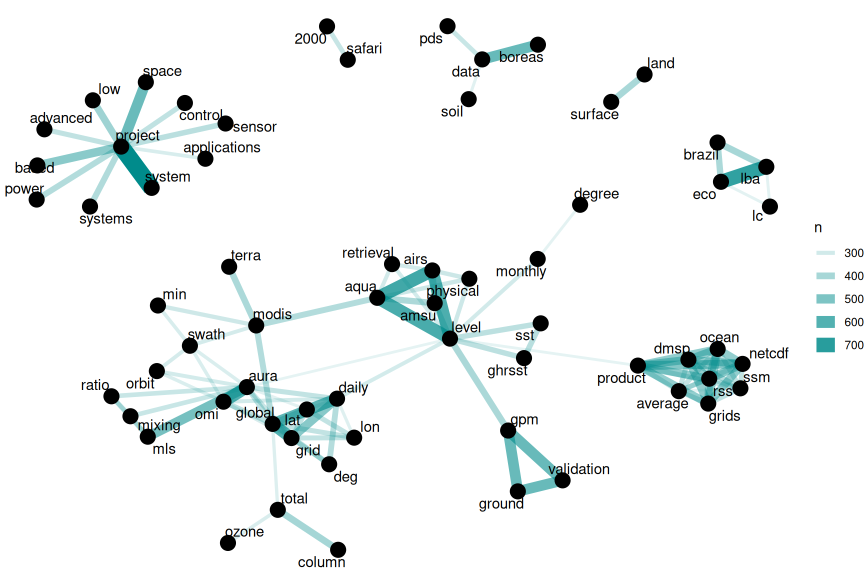
Figure 8.1: Word network in NASA dataset titles
We see some clear clustering in this network of title words; words in NASA dataset titles are largely organized into several families of words that tend to go together.
What about the words from the description fields?
set.seed(1234)
desc_word_pairs %>%
  filter(n >= 5000) %>%
  graph_from_data_frame() %>%
  ggraph(layout = "fr") +
  geom_edge_link(aes(edge_alpha = n, edge_width = n), edge_colour = "darkred") +
  geom_node_point(size = 5) +
  geom_node_text(aes(label = name), repel = TRUE,
                 point.padding = unit(0.2, "lines")) +
  theme_void()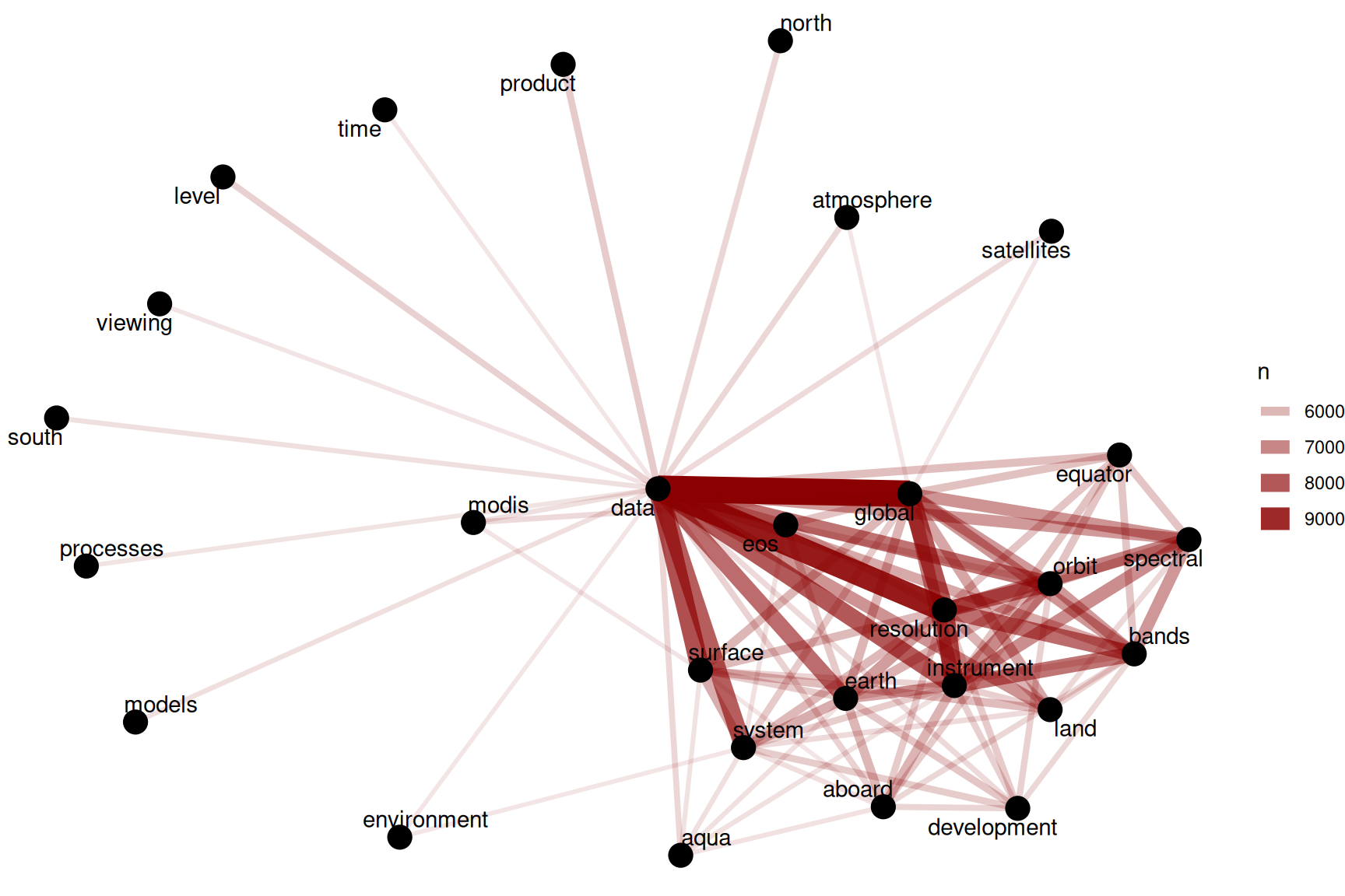
Figure 8.2: Word network in NASA dataset descriptions
Figure 8.2 shows such strong connections between the top dozen or so words (words like “data”, “global”, “resolution”, and “instrument”) that we do not see clear clustering structure in the network. We may want to use tf-idf (as described in detail in Chapter 3) as a metric to find characteristic words for each description field, instead of looking at counts of words.
8.2.2 Networks of Keywords
Next, let’s make a network of the keywords in Figure 8.3 to see which keywords commonly occur together in the same datasets.
keyword_pairs <- nasa_keyword %>%
  pairwise_count(keyword, id, sort = TRUE, upper = FALSE)

keyword_pairs
#> # A tibble: 13,390 × 3
#>    item1         item2                       n
#>    <chr>         <chr>                   <dbl>
#>  1 OCEANS        OCEAN OPTICS             7324
#>  2 EARTH SCIENCE ATMOSPHERE               7318
#>  3 OCEANS        OCEAN COLOR              7270
#>  4 OCEAN OPTICS  OCEAN COLOR              7270
#>  5 PROJECT       COMPLETED                6450
#>  6 EARTH SCIENCE ATMOSPHERIC WATER VAPOR  3142
#>  7 ATMOSPHERE    ATMOSPHERIC WATER VAPOR  3142
#>  8 EARTH SCIENCE OCEANS                   2762
#>  9 EARTH SCIENCE LAND SURFACE             2718
#> 10 EARTH SCIENCE BIOSPHERE                2448
#> # ℹ 13,380 more rows

set.seed(1234)
keyword_pairs %>%
  filter(n >= 700) %>%
  graph_from_data_frame() %>%
  ggraph(layout = "fr") +
  geom_edge_link(aes(edge_alpha = n, edge_width = n), edge_colour = "royalblue") +
  geom_node_point(size = 5) +
  geom_node_text(aes(label = name), repel = TRUE,
                 point.padding = unit(0.2, "lines")) +
  theme_void()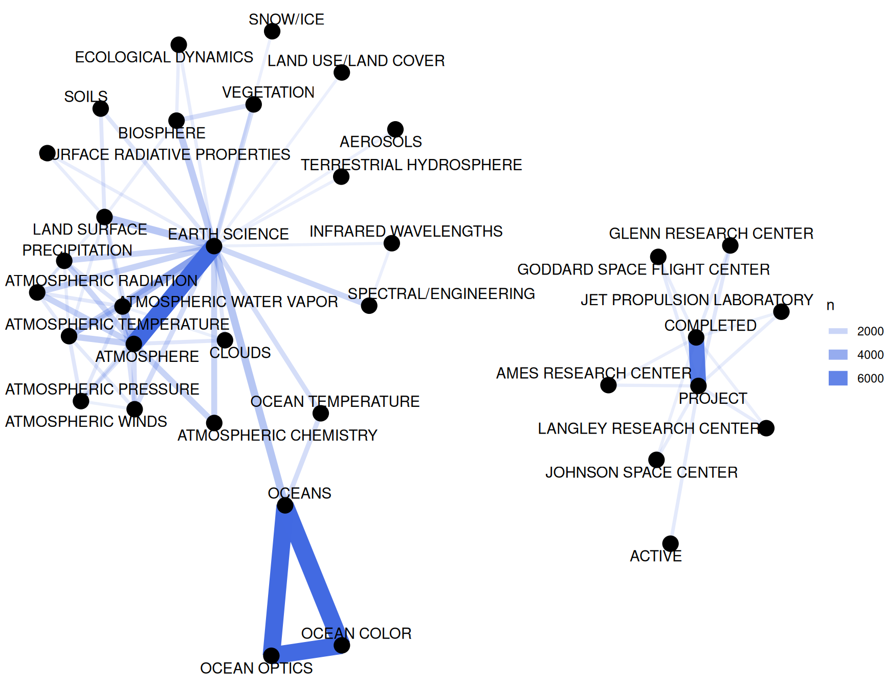
Figure 8.3: Co-occurrence network in NASA dataset keywords
We definitely see clustering here, and strong connections between keywords like “OCEANS”, “OCEAN OPTICS”, and “OCEAN COLOR”, or “PROJECT” and “COMPLETED”.
These are the most commonly co-occurring words, but also just the most common keywords in general.
To examine the relationships among keywords in a different way, we can find the correlation among the keywords as described in Chapter 4. This looks for those keywords that are more likely to occur together than with other keywords for a dataset.
keyword_cors <- nasa_keyword %>%
  group_by(keyword) %>%
  filter(n() >= 50) %>%
  pairwise_cor(keyword, id, sort = TRUE, upper = FALSE)

keyword_cors
#> # A tibble: 7,875 × 3
#>    item1               item2       correlation
#>    <chr>               <chr>             <dbl>
#>  1 KNOWLEDGE           SHARING           1
#>  2 DASHLINK            AMES              1
#>  3 SCHEDULE            EXPEDITION        1
#>  4 TURBULENCE          MODELS            0.997
#>  5 APPEL               KNOWLEDGE         0.997
#>  6 APPEL               SHARING           0.997
#>  7 OCEAN OPTICS        OCEAN COLOR       0.995
#>  8 ATMOSPHERIC SCIENCE CLOUD             0.994
#>  9 LAUNCH              SCHEDULE          0.984
#> 10 LAUNCH              EXPEDITION        0.984
#> # ℹ 7,865 more rows
Notice that these keywords at the top of this sorted data frame have correlation coefficients equal to 1; they always occur together. This means these are redundant keywords. It may not make sense to continue to use both of the keywords in these sets of pairs; instead, just one keyword could be used.
Let’s visualize the network of keyword correlations, just as we did for keyword co-occurences.
set.seed(1234)
keyword_cors %>%
  filter(correlation > .6) %>%
  graph_from_data_frame() %>%
  ggraph(layout = "fr") +
  geom_edge_link(aes(edge_alpha = correlation, edge_width = correlation), edge_colour = "royalblue") +
  geom_node_point(size = 5) +
  geom_node_text(aes(label = name), repel = TRUE,
                 point.padding = unit(0.2, "lines")) +
  theme_void()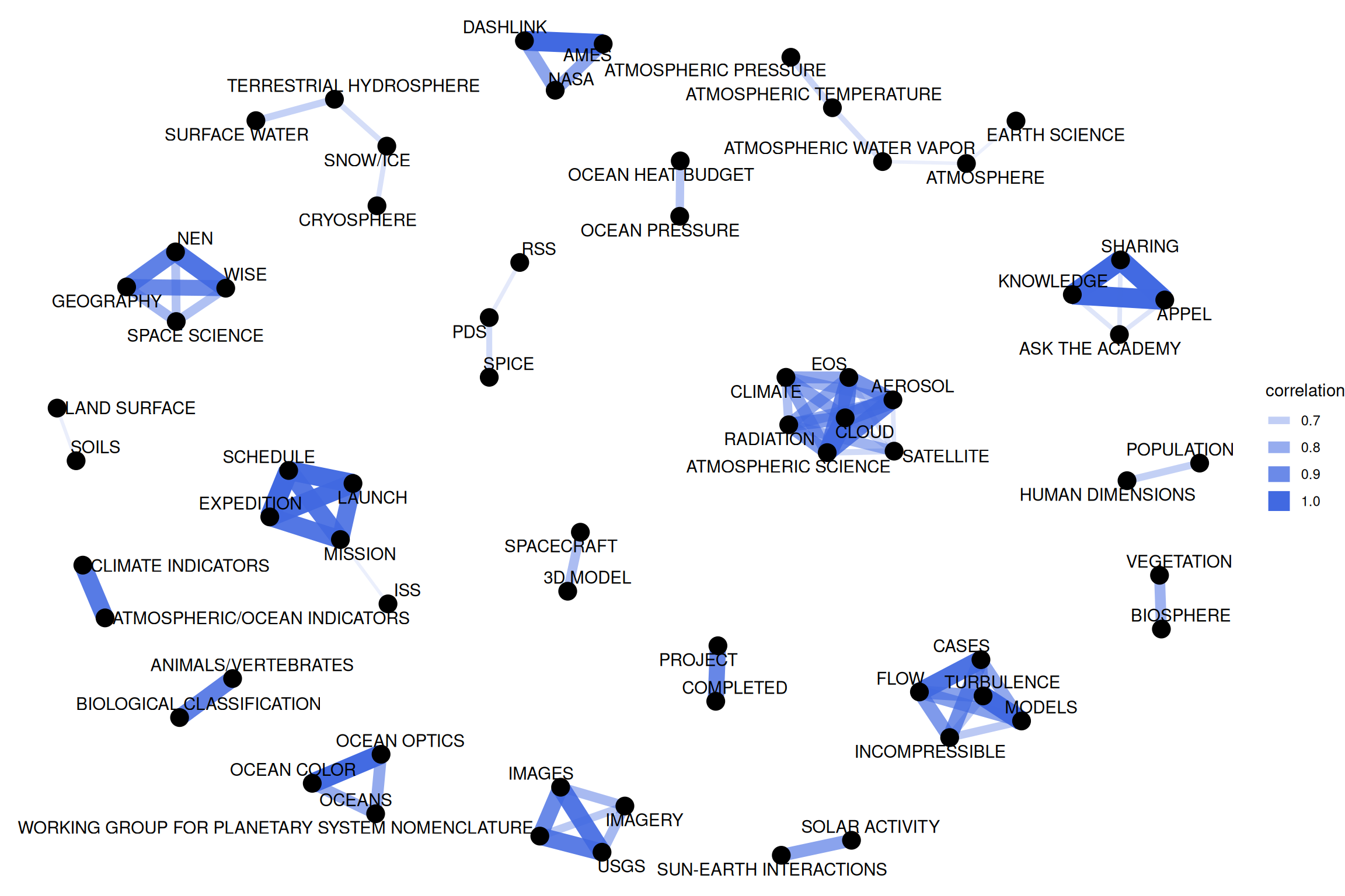
Figure 8.4: Correlation network in NASA dataset keywords
This network in Figure 8.4 appears much different than the co-occurence network. The difference is that the co-occurrence network asks a question about which keyword pairs occur most often, and the correlation network asks a question about which keywords occur more often together than with other keywords. Notice here the high number of small clusters of keywords; the network structure can be extracted (for further analysis) from the graph_from_data_frame() function above.
8.3 Calculating tf-idf for the description fields
The network graph in Figure 8.2 showed us that the description fields are dominated by a few common words like “data”, “global”, and “resolution”; this would be an excellent opportunity to use tf-idf as a statistic to find characteristic words for individual description fields. As discussed in Chapter 3, we can use tf-idf, the term frequency times inverse document frequency, to identify words that are especially important to a document within a collection of documents. Let’s apply that approach to the description fields of these NASA datasets.
8.3.1 What is tf-idf for the description field words?
We will consider each description field a document, and the whole set of description fields the collection or corpus of documents. We have already used unnest_tokens() earlier in this chapter to make a tidy data frame of the words in the description fields, so now we can use bind_tf_idf() to calculate tf-idf for each word.
desc_tf_idf <- nasa_desc %>%
  count(id, word, sort = TRUE) %>%
  bind_tf_idf(word, id, n)
What are the highest tf-idf words in the NASA description fields?
desc_tf_idf %>%
  arrange(-tf_idf)
#> # A tibble: 1,914,170 × 6
#>    id                       word                            n    tf   idf tf_idf
#>    <chr>                    <chr>                       <int> <dbl> <dbl>  <dbl>
#>  1 55942a7cc63a7fe59b49774a rdr                             1     1 10.4   10.4
#>  2 55942ac9c63a7fe59b49b688 palsar_radiometric_terrain…     1     1 10.4   10.4
#>  3 55942ac9c63a7fe59b49b689 palsar_radiometric_terrain…     1     1 10.4   10.4
#>  4 55942a7bc63a7fe59b4976ca lgrs                            1     1  8.77   8.77
#>  5 55942a7bc63a7fe59b4976d2 lgrs                            1     1  8.77   8.77
#>  6 55942a7bc63a7fe59b4976e3 lgrs                            1     1  8.77   8.77
#>  7 55942a7dc63a7fe59b497820 mri                             1     1  8.58   8.58
#>  8 55942ad8c63a7fe59b49cf6c template_proddescription        1     1  8.30   8.30
#>  9 55942ad8c63a7fe59b49cf6d template_proddescription        1     1  8.30   8.30
#> 10 55942ad8c63a7fe59b49cf6e template_proddescription        1     1  8.30   8.30
#> # ℹ 1,914,160 more rows
These are the most important words in the description fields as measured by tf-idf, meaning they are common but not too common.
Notice we have run into an issue here; both \(n\) and term frequency are equal to 1 for these terms, meaning that these were description fields that only had a single word in them. If a description field only contains one word, the tf-idf algorithm will think that is a very important word.
Depending on our analytic goals, it might be a good idea to throw out all description fields that have very few words.
8.3.2 Connecting description fields to keywords
We now know which words in the descriptions have high tf-idf, and we also have labels for these descriptions in the keywords. Let’s do a full join of the keyword data frame and the data frame of description words with tf-idf, and then find the highest tf-idf words for a given keyword.
desc_tf_idf <- full_join(desc_tf_idf, nasa_keyword, by = "id")Let’s plot some of the most important words, as measured by tf-idf, for a few example keywords used on NASA datasets. First, let’s use dplyr operations to filter for the keywords we want to examine and take just the top 15 words for each keyword. Then, let’s plot those words in Figure 8.5.
desc_tf_idf %>%
  filter(!near(tf, 1)) %>%
  filter(keyword %in% c("SOLAR ACTIVITY", "CLOUDS",
                        "SEISMOLOGY", "ASTROPHYSICS",
                        "HUMAN HEALTH", "BUDGET")) %>%
  arrange(desc(tf_idf)) %>%
  group_by(keyword) %>%
  distinct(word, keyword, .keep_all = TRUE) %>%
  slice_max(tf_idf, n = 15, with_ties = FALSE) %>%
  ungroup() %>%
  mutate(word = factor(word, levels = rev(unique(word)))) %>%
  ggplot(aes(tf_idf, word, fill = keyword)) +
  geom_col(show.legend = FALSE) +
  facet_wrap(~keyword, ncol = 3, scales = "free") +
  labs(title = "Highest tf-idf words in NASA metadata description fields",
       caption = "NASA metadata from https://data.nasa.gov/data.json",
       x = "tf-idf", y = NULL)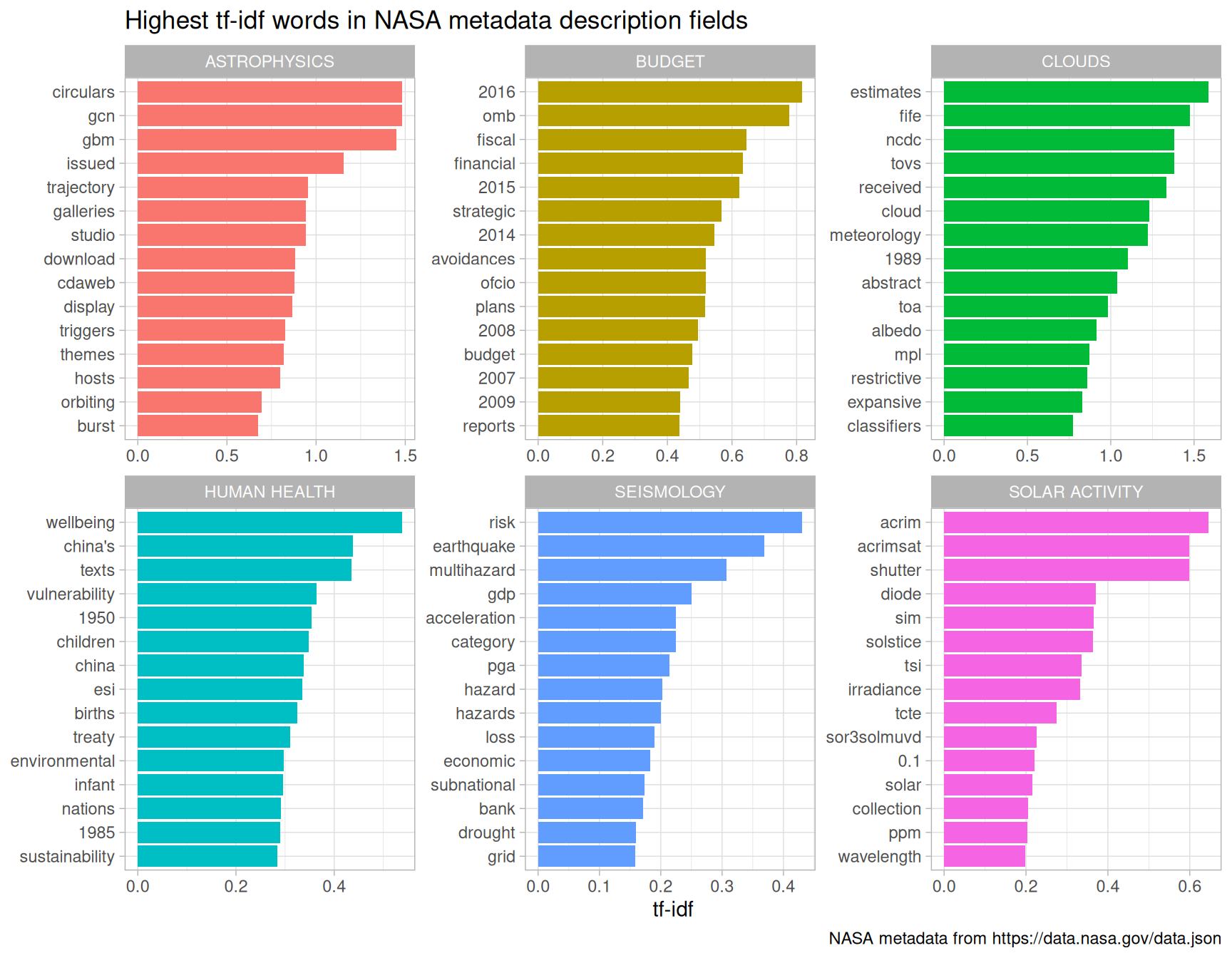
Figure 8.5: Distribution of tf-idf for words from datasets labeled with selected keywords
Using tf-idf has allowed us to identify important description words for each of these keywords. Datasets labeled with the keyword “SEISMOLOGY” have words like “earthquake”, “risk”, and “hazard” in their description, while those labeled with “HUMAN HEALTH” have descriptions characterized by words like “wellbeing”, “vulnerability”, and “children.” Most of the combinations of letters that are not English words are certainly acronyms (like OMB for the Office of Management and Budget), and the examples of years and numbers are important for these topics. The tf-idf statistic has identified the kinds of words it is intended to, important words for individual documents within a collection of documents.
8.4 Topic modeling
Using tf-idf as a statistic has already given us insight into the content of NASA description fields, but let’s try an additional approach to the question of what the NASA descriptions fields are about. We can use topic modeling as described in Chapter 6 to model each document (description field) as a mixture of topics and each topic as a mixture of words. As in earlier chapters, we will use latent Dirichlet allocation (LDA) for our topic modeling; there are other possible approaches for topic modeling.
8.4.1 Casting to a document-term matrix
To do the topic modeling as implemented here, we need to make a DocumentTermMatrix, a special kind of matrix from the tm package (of course, this is just a specific implementation of the general concept of a “document-term matrix”). Rows correspond to documents (description texts in our case) and columns correspond to terms (i.e., words); it is a sparse matrix and the values are word counts.
Let’s clean up the text a bit using stop words to remove some of the nonsense “words” leftover from HTML or other character encoding. We can use bind_rows() to add our custom stop words to the list of default stop words from the tidytext package, and then all at once use anti_join() to remove them all from our data frame.
my_stop_words <- bind_rows(stop_words,
                           tibble(word = c("nbsp", "amp", "gt", "lt",
                                           "timesnewromanpsmt", "font",
                                           "td", "li", "br", "tr", "quot",
                                           "st", "img", "src", "strong",
                                           "http", "file", "files",
                                           as.character(1:12)),
                                  lexicon = rep("custom", 30)))

word_counts <- nasa_desc %>%
  anti_join(my_stop_words) %>%
  count(id, word, sort = TRUE) %>%
  ungroup()

word_counts
#> # A tibble: 1,896,211 × 3
#>    id                       word         n
#>    <chr>                    <chr>    <int>
#>  1 55942a8ec63a7fe59b4986ef suit        82
#>  2 55942a8ec63a7fe59b4986ef space       69
#>  3 56cf5b00a759fdadc44e564a data        41
#>  4 56cf5b00a759fdadc44e564a leak        40
#>  5 56cf5b00a759fdadc44e564a tree        39
#>  6 55942a8ec63a7fe59b4986ef pressure    34
#>  7 55942a8ec63a7fe59b4986ef system      34
#>  8 55942a89c63a7fe59b4982d9 em          32
#>  9 55942a8ec63a7fe59b4986ef al          32
#> 10 55942a8ec63a7fe59b4986ef human       31
#> # ℹ 1,896,201 more rows
This is the information we need, the number of times each word is used in each document, to make a DocumentTermMatrix. We can cast() from our tidy text format to this non-tidy format as described in detail in Chapter 5.
desc_dtm <- word_counts %>%
  cast_dtm(id, word, n)

desc_dtm
#> <<DocumentTermMatrix (documents: 32003, terms: 35336)>>
#> Non-/sparse entries: 1896211/1128961797
#> Sparsity           : 100%
#> Maximal term length: 166
#> Weighting          : term frequency (tf)
We see that this dataset contains documents (each of them a NASA description field) and terms (words). Notice that this example document-term matrix is (very close to) 100% sparse, meaning that almost all of the entries in this matrix are zero. Each non-zero entry corresponds to a certain word appearing in a certain document.
8.4.2 Ready for topic modeling
Now let’s use the topicmodels package to create an LDA model. How many topics will we tell the algorithm to make? This is a question much like in \(k\)-means clustering; we don’t really know ahead of time. We tried the following modeling procedure using 8, 16, 24, 32, and 64 topics; we found that at 24 topics, documents are still getting sorted into topics cleanly but going much beyond that caused the distributions of \(\gamma\), the probability that each document belongs in each topic, to look worrisome. We will show more details on this later.
library(topicmodels)

# be aware that running this model is time intensive
desc_lda <- LDA(desc_dtm, k = 24, control = list(seed = 1234))
desc_lda
#> A LDA_VEM topic model with 24 topics.This is a stochastic algorithm that could have different results depending on where the algorithm starts, so we need to specify a seed for reproducibility as shown here.
8.4.3 Interpreting the topic model
Now that we have built the model, let’s tidy() the results of the model, i.e., construct a tidy data frame that summarizes the results of the model. The tidytext package includes a tidying method for LDA models from the topicmodels package.
tidy_lda <- tidy(desc_lda)

tidy_lda
#> # A tibble: 861,624 × 3
#>    topic term       beta
#>    <int> <chr>     <dbl>
#>  1     1 suit  1.00e-121
#>  2     2 suit  2.63e-145
#>  3     3 suit  1.92e- 79
#>  4     4 suit  6.72e- 45
#>  5     5 suit  1.74e- 85
#>  6     6 suit  7.69e- 84
#>  7     7 suit  3.28e-  4
#>  8     8 suit  3.74e- 20
#>  9     9 suit  4.85e- 15
#> 10    10 suit  4.77e- 10
#> # ℹ 861,614 more rows
The column \(\beta\) tells us the probability of that term being generated from that topic for that document. It is the probability of that term (word) belonging to that topic. Notice that some of the values for \(\beta\) are very, very low, and some are not so low.
What is each topic about? Let’s examine the top 10 terms for each topic.
top_terms <- tidy_lda %>%
  group_by(topic) %>%
  slice_max(beta, n = 10, with_ties = FALSE) %>%
  ungroup() %>%
  arrange(topic, -beta)

top_terms
#> # A tibble: 240 × 3
#>    topic term          beta
#>    <int> <chr>        <dbl>
#>  1     1 data        0.0449
#>  2     1 soil        0.0368
#>  3     1 moisture    0.0295
#>  4     1 amsr        0.0244
#>  5     1 sst         0.0168
#>  6     1 validation  0.0132
#>  7     1 temperature 0.0132
#>  8     1 surface     0.0129
#>  9     1 accuracy    0.0123
#> 10     1 set         0.0116
#> # ℹ 230 more rows
It is not very easy to interpret what the topics are about from a data frame like this so let’s look at this information visually in Figure 8.6.
top_terms %>%
  mutate(term = reorder_within(term, beta, topic)) %>%
  group_by(topic, term) %>%
  arrange(desc(beta)) %>%
  ungroup() %>%
  ggplot(aes(beta, term, fill = as.factor(topic))) +
  geom_col(show.legend = FALSE) +
  scale_y_reordered() +
  labs(title = "Top 10 terms in each LDA topic",
       x = expression(beta), y = NULL) +
  facet_wrap(~ topic, ncol = 4, scales = "free")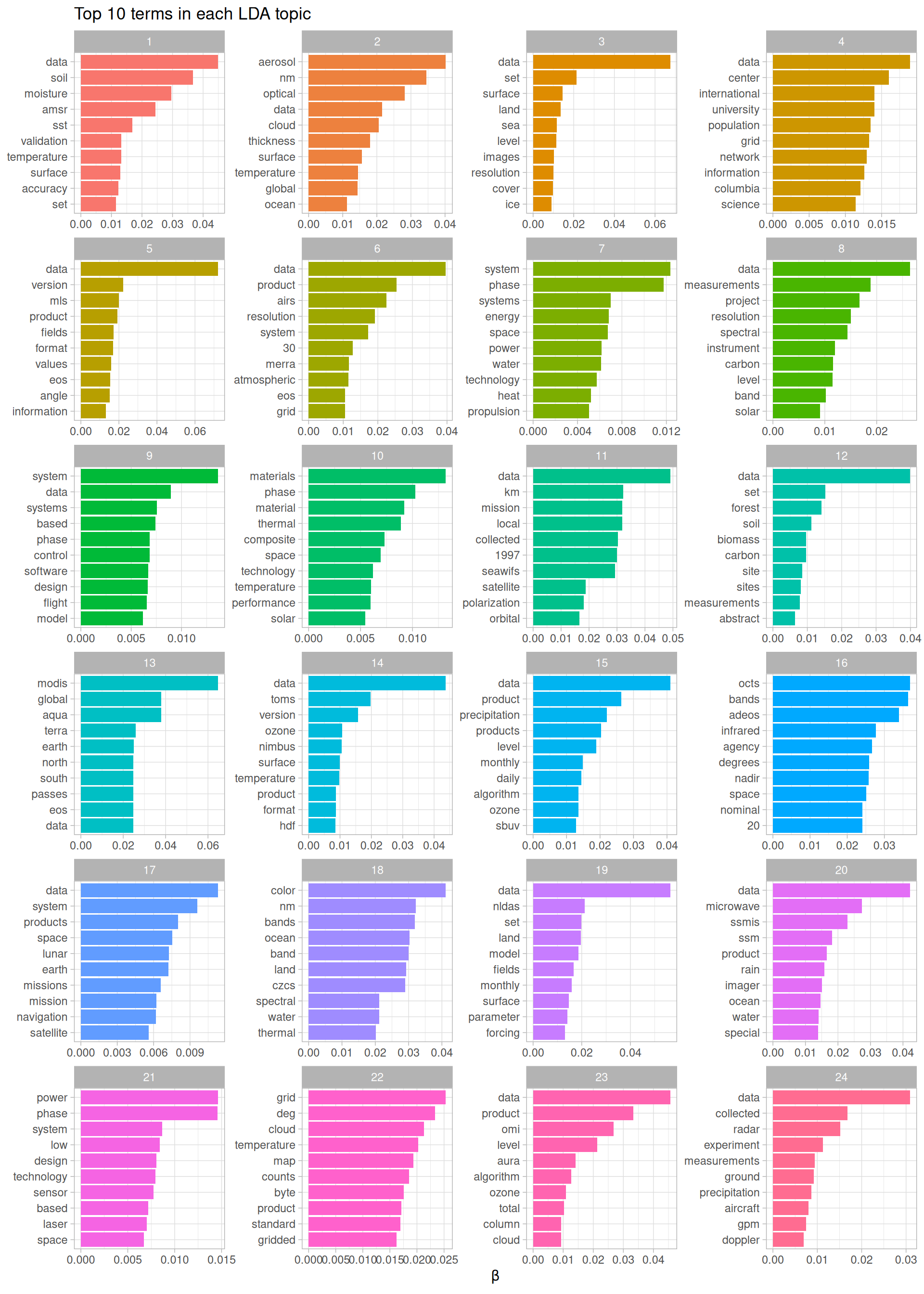
Figure 8.6: Top terms in topic modeling of NASA metadata description field texts
We can see what a dominant word “data” is in these description texts. In addition, there are meaningful differences between these collections of terms, from terms about soil, forests, and biomass in topic 12 to terms about design, systems, and technology in topic 21. The topic modeling process has identified groupings of terms that we can understand as human readers of these description fields.
We just explored which words are associated with which topics. Next, let’s examine which topics are associated with which description fields (i.e., documents). We will look at a different probability for this, \(\gamma\), the probability that each document belongs in each topic, again using the tidy verb.
lda_gamma <- tidy(desc_lda, matrix = "gamma")

lda_gamma
#> # A tibble: 768,072 × 3
#>    document                 topic      gamma
#>    <chr>                    <int>      <dbl>
#>  1 55942a8ec63a7fe59b4986ef     1 0.00000645
#>  2 56cf5b00a759fdadc44e564a     1 0.0000116
#>  3 55942a89c63a7fe59b4982d9     1 0.0492
#>  4 56cf5b00a759fdadc44e55cd     1 0.0000225
#>  5 55942a89c63a7fe59b4982c6     1 0.0000661
#>  6 55942a86c63a7fe59b498077     1 0.0000567
#>  7 56cf5b00a759fdadc44e56f8     1 0.0000475
#>  8 55942a8bc63a7fe59b4984b5     1 0.0000431
#>  9 55942a6ec63a7fe59b496bf7     1 0.0000441
#> 10 55942a8ec63a7fe59b4986f6     1 0.0000288
#> # ℹ 768,062 more rows
Notice that some of the probabilities visible at the top of the data frame are low and some are higher. Our model has assigned a probability to each description belonging to each of the topics we constructed from the sets of words. How are the probabilities distributed? Let’s visualize them (Figure 8.7).
ggplot(lda_gamma, aes(gamma)) +
  geom_histogram(alpha = 0.8) +
  scale_y_log10() +
  labs(title = "Distribution of probabilities for all topics",
       y = "Number of documents", x = expression(gamma))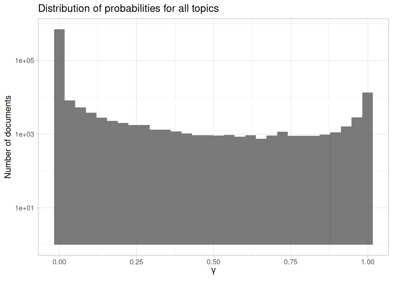
Figure 8.7: Probability distribution in topic modeling of NASA metadata description field texts
First notice that the y-axis is plotted on a log scale; otherwise it is difficult to make out any detail in the plot. Next, notice that \(\gamma\) runs from 0 to 1; remember that this is the probability that a given document belongs in a given topic. There are many values near zero, which means there are many documents that do not belong in each topic. Also, there are many values near \(\gamma = 1\); these are the documents that do belong in those topics. This distribution shows that documents are being well discriminated as belonging to a topic or not. We can also look at how the probabilities are distributed within each topic, as shown in Figure 8.8.
ggplot(lda_gamma, aes(gamma, fill = as.factor(topic))) +
  geom_histogram(alpha = 0.8, show.legend = FALSE) +
  facet_wrap(~ topic, ncol = 4) +
  scale_y_log10() +
  labs(title = "Distribution of probability for each topic",
       y = "Number of documents", x = expression(gamma))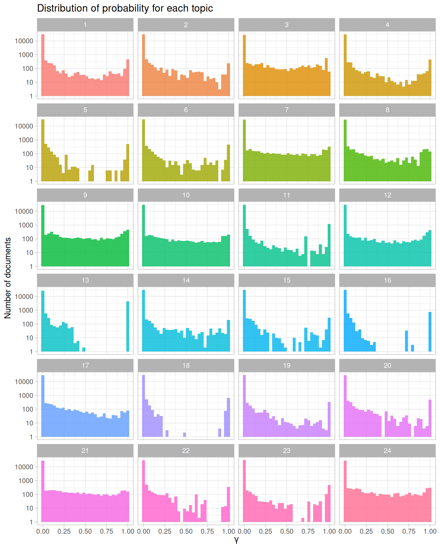
Figure 8.8: Probability distribution for each topic in topic modeling of NASA metadata description field texts
Let’s look specifically at topic 18 in Figure 8.8, a topic that had documents cleanly sorted in and out of it. There are many documents with \(\gamma\) close to 1; these are the documents that do belong to topic 18 according to the model. There are also many documents with \(\gamma\) close to 0; these are the documents that do not belong to topic 18. Each document appears in each panel in this plot, and its \(\gamma\) for that topic tells us that document’s probability of belonging in that topic.
This plot displays the type of information we used to choose how many topics for our topic modeling procedure. When we tried options higher than 24 (such as 32 or 64), the distributions for \(\gamma\) started to look very flat toward \(\gamma = 1\); documents were not getting sorted into topics very well.
8.4.4 Connecting topic modeling with keywords
Let’s connect these topic models with the keywords and see what relationships we can find. We can full_join() this to the human-tagged keywords and discover which keywords are associated with which topic.
lda_gamma <- full_join(lda_gamma, nasa_keyword, by = c("document" = "id"))

lda_gamma
#> # A tibble: 3,037,671 × 4
#>    document                 topic      gamma keyword
#>    <chr>                    <int>      <dbl> <chr>
#>  1 55942a8ec63a7fe59b4986ef     1 0.00000645 JOHNSON SPACE CENTER
#>  2 55942a8ec63a7fe59b4986ef     1 0.00000645 PROJECT
#>  3 55942a8ec63a7fe59b4986ef     1 0.00000645 COMPLETED
#>  4 56cf5b00a759fdadc44e564a     1 0.0000116  DASHLINK
#>  5 56cf5b00a759fdadc44e564a     1 0.0000116  AMES
#>  6 56cf5b00a759fdadc44e564a     1 0.0000116  NASA
#>  7 55942a89c63a7fe59b4982d9     1 0.0492     GODDARD SPACE FLIGHT CENTER
#>  8 55942a89c63a7fe59b4982d9     1 0.0492     PROJECT
#>  9 55942a89c63a7fe59b4982d9     1 0.0492     COMPLETED
#> 10 56cf5b00a759fdadc44e55cd     1 0.0000225  DASHLINK
#> # ℹ 3,037,661 more rows
Now we can use filter() to keep only the document-topic entries that have probabilities (\(\gamma\)) greater than some cut-off value; let’s use 0.9.
top_keywords <- lda_gamma %>%
  filter(gamma > 0.9) %>%
  count(topic, keyword, sort = TRUE)

top_keywords
#> # A tibble: 1,022 × 3
#>    topic keyword           n
#>    <int> <chr>         <int>
#>  1    13 OCEAN COLOR    4480
#>  2    13 OCEAN OPTICS   4480
#>  3    13 OCEANS         4480
#>  4    11 OCEAN COLOR    1216
#>  5    11 OCEAN OPTICS   1216
#>  6    11 OCEANS         1216
#>  7     9 PROJECT         926
#>  8    12 EARTH SCIENCE   909
#>  9     9 COMPLETED       834
#> 10    16 OCEAN COLOR     768
#> # ℹ 1,012 more rows
What are the top keywords for each topic?
top_keywords %>%
  group_by(topic) %>%
  slice_max(n, n = 5, with_ties = FALSE) %>%
  ungroup %>%
  mutate(keyword = reorder_within(keyword, n, topic)) %>%
  ggplot(aes(n, keyword, fill = as.factor(topic))) +
  geom_col(show.legend = FALSE) +
  labs(title = "Top keywords for each LDA topic",
       x = "Number of documents", y = NULL) +
  scale_y_reordered() +
  facet_wrap(~ topic, ncol = 4, scales = "free")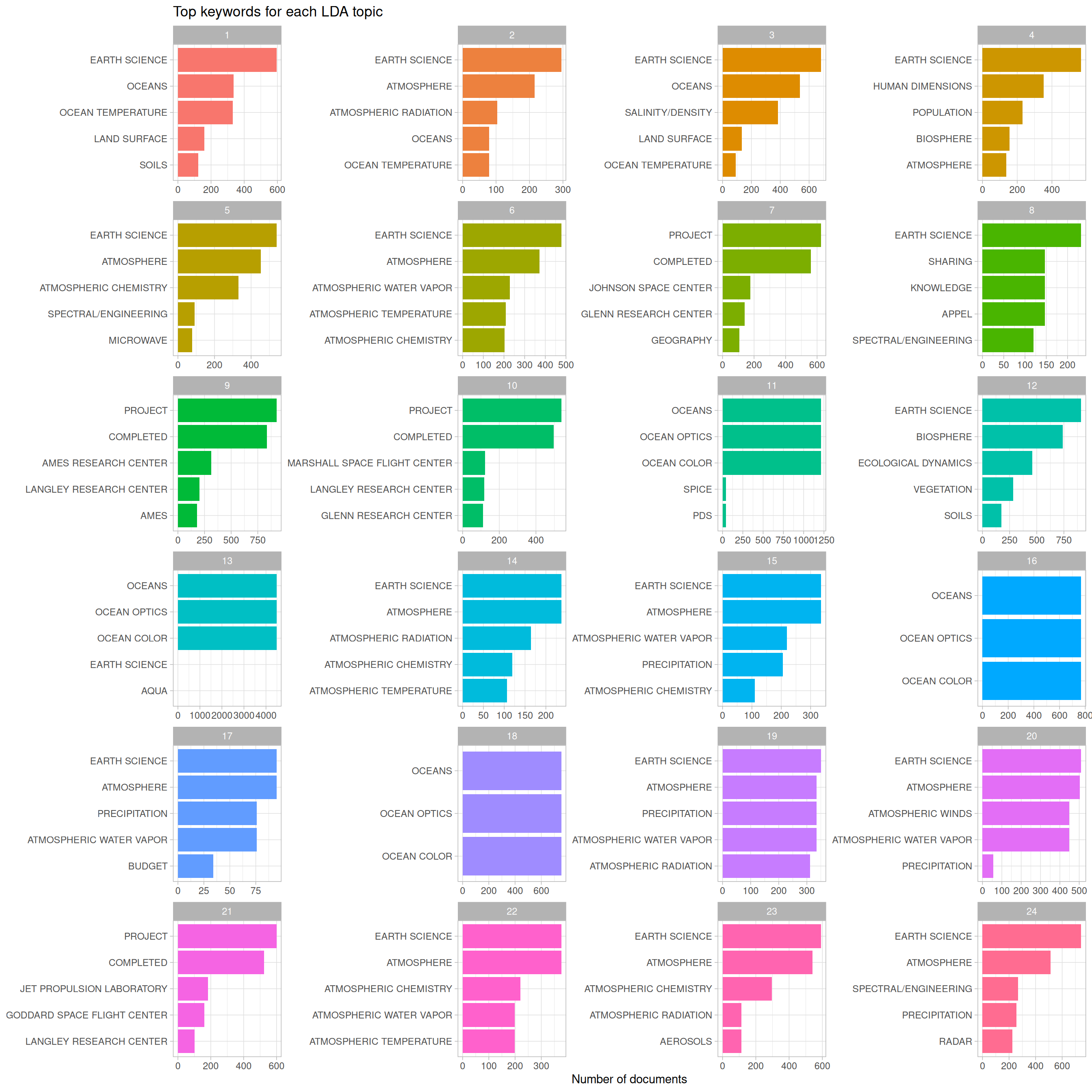
Figure 8.9: Top keywords in topic modeling of NASA metadata description field texts
Let’s take a step back and remind ourselves what Figure 8.9 is telling us. NASA datasets are tagged with keywords by human beings, and we have built an LDA topic model (with 24 topics) for the description fields of the NASA datasets. This plot answers the question, “For the datasets with description fields that have a high probability of belonging to a given topic, what are the most common human-assigned keywords?”
It’s interesting that the keywords for topics 13, 16, and 18 are essentially duplicates of each other (“OCEAN COLOR”, “OCEAN OPTICS”, “OCEANS”), because the top words in those topics do exhibit meaningful differences, as shown in Figure 8.6. Also note that by number of documents, the combination of 13, 16, and 18 is quite a large percentage of the total number of datasets represented in this plot, and even more if we were to include topic 11. By number, there are many datasets at NASA that deal with oceans, ocean color, and ocean optics. We see “PROJECT COMPLETED” in topics 9, 10, and 21, along with the names of NASA laboratories and research centers. Other important subject areas that stand out are groups of keywords about atmospheric science, budget/finance, and population/human dimensions. We can go back to Figure 8.6 on terms and topics to see which words in the description fields are driving datasets being assigned to these topics. For example, topic 4 is associated with keywords about population and human dimensions, and some of the top terms for that topic are “population”, “international”, “center”, and “university”.
8.5 Summary
By using a combination of network analysis, tf-idf, and topic modeling, we have come to a greater understanding of how datasets are related at NASA. Specifically, we have more information now about how keywords are connected to each other and which datasets are likely to be related. The topic model could be used to suggest keywords based on the words in the description field, or the work on the keywords could suggest the most important combination of keywords for certain areas of study.